Root mean square deviation standard deviation

Asked by: Chandler Ritchie

Physical scientists often use the term root mean square as a synonym for standard deviation when it can be assumed the input signal has zero mean, that is, referring to the square root of the mean squared deviation of a signal from a given baseline or fit.

While measures of central tendency are used to estimate «normal» values of
a dataset, measures of dispersion are important for describing the spread of the
data, or its variation around a central value.
Two distinct samples may have the same
mean or
median, but completely different levels of variability, or vice versa. A proper
description of a set of data should include both of these characteristics. There
are various methods that can be used to measure the dispersion of a dataset, each
with its own set of advantages and
disadvantages.

Facts about Standard Deviation

Table 1 illustrates the difference between standard deviation and the RMSE in revealing the presence of biases in measurements. The table represents a vertical accuracy evaluation for points cloud derived from UAS imagery by comparing it to a higher accuracy elevation model derived from a mobile lidar mapping system. The UAS-derived elevation model needed to meet 5-cm (0.164-ft) accuracy. If we used standard deviation alone, the data would meet the specifications with a value of 0.076-ft. However, looking at the high value of 0.246-ft. (7.5-cm) of the mean, it is obvious this data set contains a bias and the only way to catch it is by either evaluating the value of the mean or using the RMSE as the accuracy measure. The high value of the RMSE = 0.257-ft. (7.83-cm) will flag the data as not meeting specifications. The far right column contains the error values after removing the bias of  0.246-ft. (7.5-cm) from the measurements. Once we remove the bias, the values for the RMSE and the standard deviation are equal and they both meet the project accuracy specifications. Removing a bias from elevation data could be as simple as shifting the entire dataset up or down by the magnitude of the bias itself, such practice is called z-pump.

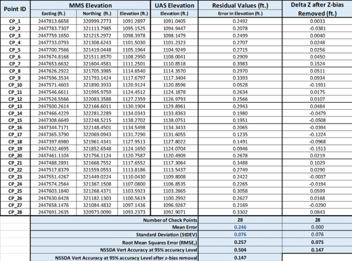
Table 1 Vertical Accuracy Tabulation of Geospatial Product

Click for a text description of Table 1.

Let’s try to explore why this measure of error makes sense from a mathematical perspective. Ignoring the division by n under the square root, the first thing we can notice is a resemblance to the formula for the Euclidean distance between two vectors in ℝⁿ:

This tells us heuristically that RMSE can be thought of as some kind of (normalized) distance between the vector of predicted values and the vector of observed values.

But why are we dividing by n under the square root here? If we keep n (the number of observations) fixed, all it does is rescale the Euclidean distance by a factor of √(1/n). It’s a bit tricky to see why this is the right thing to do, so let’s delve in a bit deeper.

These errors, thought of as random variables, might have Gaussian distribution with mean μ and standard deviation σ, but any other distribution with a square-integrable PDF (probability density function) would also work. We want to think of ŷᵢ as an underlying physical quantity, such as the exact distance from Mars to the Sun at a particular point in time. Our observed quantity yᵢ would then be the distance from Mars to the Sun as we measure it, with some errors coming from mis-calibration of our telescopes and measurement noise from atmospheric interference.

(NOT TO SCALE)

The mean μ of the distribution of our errors would correspond to a persistent bias coming from mis-calibration, while the standard deviation σ would correspond to the amount of measurement noise. Imagine now that we know the mean μ of the distribution for our errors exactly and would like to estimate the standard deviation σ. We can see through a bit of calculation that:

Remember that we assumed we already knew μ exactly. That is, the persistent bias in our instruments is a known bias, rather than an unknown bias. So we might as well correct for this bias right off the bat by subtracting μ from all our raw observations. That is, we might as well suppose our errors are already distributed with mean μ = 0. Plugging this into the equation above and taking the square root of both sides then yields:

We should also now have an explanation for the division by n under the square root in RMSE: it allows us to estimate the standard deviation σ of the error for a typical single observation rather than some kind of “total error”. By dividing by n, we keep this measure of error consistent as we move from a small collection of observations to a larger collection (it just becomes more accurate as we increase the number of observations). To phrase it another way, RMSE is a good way to answer the question: “How far off should we expect our model to be on its next prediction?”

To sum up our discussion, RMSE is a good measure to use if we want to estimate the standard deviation σ of a typical observed value from our model’s prediction, assuming that our observed data can be decomposed as:

The random noise here could be anything that our model does not capture (e.g., unknown variables that might influence the observed values). If the noise is small, as estimated by RMSE, this generally means our model is good at predicting our observed data, and if RMSE is large, this generally means our model is failing to account for important features underlying our data.

Связь стандартного отклонения со среднеквадратичными значениями

Добавлено 8 августа 2020 в 10:48

В данной статье исследуется интересная связь между важным статистическим параметром и одним из фундаментальных аналитических инструментов электротехники.

Если вы только присоединились к этой серии статей о статистике в электротехнике, возможно, вы захотите начать с первой статьи, посвященной статистическому анализу, и просмотра второй об описательной статистике. Совсем недавно мы коснулись компенсации размера выборки при вычислении стандартных отклонений, уделяя особое внимание коррекции Бесселя.

В данной статье мы будем основываться на обсуждении стандартного отклонения в предыдущей статье, которое фиксирует усредненную мощность случайных вариаций в наборе данных или в оцифрованном сигнале. Эта усредненная мощность выражается в виде амплитуды, например в вольтах, а не в ваттах.

Инженеры-электронщики постоянно имеют дело со случайными отклонениями. Мы называем их шумом, и они гарантируют, что какой бы хорошей погода ни была, нам будет на что пожаловаться.

Для расчета стандартного отклонения мы используем следующую формулу:

Среднеквадратичное значение (RMS, Root Mean Square)

Большинство из нас, вероятно, впервые узнали о значениях RMS в контексте анализа сигналов переменного тока. В системах переменного тока среднеквадратичное значение напряжения или тока часто более информативно, чем значение, определяющее пиковое напряжение или ток, потому что RMS является более прямым путем к определению рассеиваемой мощности.

Мы не можем использовать пиковое значение напряжения или тока при расчете рассеиваемой мощности, потому что напряжение или ток постоянно меняются, и, следовательно, мгновенная рассеиваемая мощность также изменяется. Расчет на основе пикового значения приведет к завышению усредненной по времени мощности.

Среднеквадратичные значения позволяют рассчитывать рассеиваемую мощность, как если бы мы работали со значениями постоянного тока. Конкретнее, среднеквадратичное значение синусоидального напряжения или тока равно амплитуде сигнала постоянного напряжения или тока, которая создаст такое же количество усредненной по времени рассеиваемой мощности.

Батарея 12 В, подключенная к резистору 10 Ом, будет генерировать 122/10 = 14,4 Вт (мгновенной и средней) мощности. Если мы заменим батарею на источник переменного напряжения со среднеквадратичным значением напряжения 12 В, (средняя) мощность будет такой же.

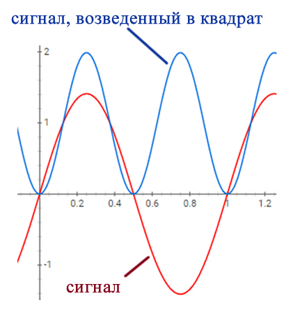
Рисунок 1 – Здесь мы вычисляем среднеквадратичное значение синусоидального сигнала, разделив пиковое значение на √2.

Мощность пропорциональна квадрату напряжения или тока. Постоянное напряжение 1 В, поданное на цепь с сопротивлением R, будет создавать 12/R=1/R Вт мощности. Взглянув на рисунок выше, мы можем видеть, что синяя кривая имеет среднее значение 1; таким образом, поскольку синяя кривая равна квадрату красной кривой, средняя мощность, генерируемая красной кривой, также будет равна 1/R.

Полный расчет среднеквадратичного значения (RMS)

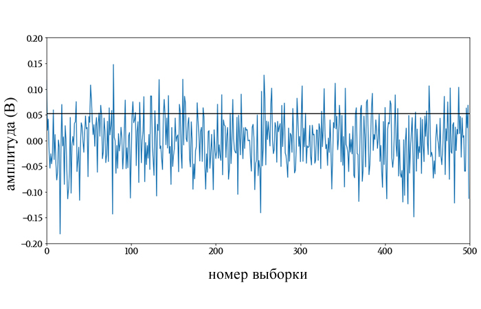
Рисунок 2 – Горизонтальная линия указывает среднеквадратичное значение этого шумового сигнала. Пиковое значение случайного шума обычно в 3-4 раза превышает среднеквадратичное значение.

Фактическое вычисление RMS, то есть вычисление, которое мы применяем к сигналам в целом, выражается следующим образом:

Эта же процедура словами: предположим, что x(t) – это сигнал во временной области, периодический в интервале от времени T1 до времени T2. Мы возводим в квадрат x(t), интегрируем этот возведенный в квадрат сигнал по соответствующему интервалу, делим интегрированное значение на длину интервала и затем извлекаем квадратный корень.

Интегрирование от T1 до T2 с последующим делением на (T2–T1) аналогично суммированию всех значений сигнала и делению на количество этих значений. Другими словами, выполнение этих двух шагов является эквивалентом во временной области для вычисления среднего арифметического для набора данных. Таким образом, мы извлекаем квадратный корень из среднего значения возведенного в квадрат сигнала: среднеквадратичное значение.

Среднеквадратичное значение (RMS) для дискретных данных

Как преобразовать приведенную выше формулу во что-то, что можно применить к дискретным данным? Другими словами, как мы можем вычислить среднеквадратичное значение оцифрованного сигнала?

Таким образом, мы можем записать наш расчет среднеквадратичного значения (RMS), дискретного по времени, следующим образом:

Это начинает казаться знакомым? Мы возводим значения в квадрат, суммируем их, делим на количество значений и извлекаем квадратный корень.

Есть только два отличия между этой процедурой и процедурой, которую мы используем для расчета стандартного отклонения:

Если мы пытаемся установить связь между среднеквадратичным значением и стандартным отклонением, второе различие может показаться решающим.

Однако учтите следующее: если среднее значение равно нулю, как это часто бывает в электрических сигналах, не будет никакой разницы между вычислением RMS и вычислением стандартного отклонения. Другими словами, для сигнала без смещения по постоянному току стандартное отклонение сигнала также равно среднеквадратичному значению.

Заключение

Я не собираюсь пытаться исследовать полное значение этой связи между стандартным отклонением и среднеквадратичным значением. Тем не менее, прежде чем мы закончим, я хочу упомянуть два интересных момента, которые вытекают из обсуждения выше.

Во-первых, стандартное отклонение дает нам среднеквадратичное значение сигнала «с развязкой по постоянному току»: мы можем рассчитать стандартное отклонение, когда смещение сигнала по постоянному току не имеет значения, и это дает нам среднеквадратичное значение только переменной составляющей.

Во-вторых, стандартное отклонение можно интерпретировать как количественную оценку шума, а анализ шума тесно связан со среднеквадратичным значением.

Теги

Анализ шумаСреднеквадратичное значение / RMS (root mean square value)Стандартное отклонениеШумЭлектрические системы переменного тока

Range of prediction

The range of the prediction is the maximum and minimum value in the predicted values. Even range helps us to understand the dispersion between models.

Median Absolute Deviation (MAD)

: Find the median absolute deviation of climatological monthly precipitation in South
America for January 1970 to December 2003.

Root Mean Square Anomaly / Root Mean Square

: Calculate the root mean square anomaly of monthly cloud cover over Africa for January
1960 to December 1979.

Mean/Median of prediction

We can understand the bias in prediction between two models using the arithmetic mean of the predicted values.

For example, The mean of predicted values of 0.5 API is calculated by taking the sum of the predicted values for 0.5 API divided by the total number of samples having 0.5 API.

In Fig.1, We can understand how PLS and SVR have performed wrt mean. SVR predicted 0.0 API much better than PLS, whereas, PLS predicted 3.0 API better than SVR. We can choose the models based on the interest of the API level.

Disadvantage: Mean is affected by outliers. Use Median when you have outliers in your predicted values

Fig.1. Comparing the mean of predicted values between the two models

Interquartile Range (IQR)

: Find the interquartile range of climatological monthly
precipitation in South America for January 1970 to December 2003.

Coefficient of Determination (R2)

R-squared (R2) is a statistical measure that represents the proportion of the variance for a dependent variable that’s explained by an independent variable or variables in a regression model. Whereas correlation explains the strength of the relationship between an independent and dependent variable, R-squared explains to what extent the variance of one variable explains the variance of the second variable. So, if the R2 of a model is 0.50, then approximately half of the observed variation can be explained by the model’s inputs.

R Squared formula

R (Correlation) (source: http://www.mathsisfun.com/data/correlation.html)

from sklearn.metrics import r2_scorer2_score(Actual, Predicted)

In statistics, mean absolute error (MAE) is a measure of errors between paired observations expressing the same phenomenon. Examples of Y versus X include comparisons of predicted versus observed, subsequent time versus initial time, and one technique of measurement versus an alternative technique of measurement. It has the same unit as the original data, and it can only be compared between models whose errors are measured in the same units. It is usually similar in magnitude to RMSE, but slightly smaller. MAE is calculated as:

Mean Absolute Error (MAE) Formula

from sklearn.metrics import mean_absolute_errormean_absolute_error(actual, predicted)

It is thus an arithmetic average of the absolute errors, where yi is the prediction and xi the actual value. Note that alternative formulations may include relative frequencies as weight factors. The mean absolute error uses the same scale as the data being measured. This is known as a scale-dependent accuracy measure and, therefore cannot be used to make comparisons between series using different scales.

Note: As you see, all the statistics compare true values to their estimates, but do it in a slightly different way. They all tell you “how far away” are your estimated values from the true value. Sometimes square roots are used and occasionally absolute values — this is because when using square roots, the extreme values have more influence on the result (see Why to square the difference instead of taking the absolute value in standard deviation? or on Mathoverflow).

In MAE and RMSE, you simply look at the “average difference” between those two values. So you interpret them comparing to the scale of your variable (i.e., MSE of 1 point is a difference of 1 point of actual between predicted and actual).

In RAE and Relative RSE, you divide those differences by the variation of actual, so they have a scale from 0 to 1, and if you multiply this value by 100, you get similarity in 0–100 scale (i.e. percentage).

Long answer: the ideal MSE isn’t 0, since then you would have a model that perfectly predicts your training data, but which is very unlikely to perfectly predict any other data. What you want is a balance between overfit (very low MSE for training data) and underfit (very high MSE for test/validation/unseen data).

Why is standard deviation called root mean square deviation?

Standard Deviation is also known as root-mean square deviation as it is the square root of means of the squared deviations from the arithmetic mean. In financial terms, standard deviation is used -to measure risks involved in an investment instrument.

The relative squared error (RSE) is relative to what it would have been if a simple predictor had been used. More specifically, this simple predictor is just the average of the actual values. Thus, the relative squared error takes the total squared error and normalizes it by dividing by the total squared error of the simple predictor. It can be compared between models whose errors are measured in the different units.

Mathematically, the relative squared error, Ei of an individual model i is evaluated by the equation:

Relative Squared Error (RSE) Formula

where P(ij) is the value predicted by the individual model i for record j (out of n records); Tj is the target value for record j, and Tbar is given by the formula:

For a perfect fit, the numerator is equal to 0 and Ei = 0. So, the Ei index ranges from 0 to infinity, with 0 correspondings to the ideal.

Trimmed Variance

: Find the trimmed variance of average OLR values in the eastern United States for
January 1980 to December 1999.

Subtleties of Using RMSE

In data science, RMSE has a double purpose:

This raises an important question: What does it mean for RMSE to be “small”?

We should note first and foremost that “small” will depend on our choice of units, and on the specific application we are hoping for. 100 inches is a big error in a building design, but 100 nanometers is not. On the other hand, 100 nanometers is a small error in fabricating an ice cube tray, but perhaps a big error in fabricating an integrated circuit.

For training models, it doesn’t really matter what units we are using, since all we care about during training is having a heuristic to help us decrease the error with each iteration. We care only about relative size of the error from one step to the next, not the absolute size of the error.

But in evaluating trained models in data science for usefulness / accuracy , we do care about units, because we aren’t just trying to see if we’re doing better than last time: we want to know if our model can actually help us solve a practical problem. The subtlety here is that evaluating whether RMSE is sufficiently small or not will depend on how accurate we need our model to be for our given application. There is never going to be a mathematical formula for this, because it depends on things like human intentions (“What are you intending to do with this model?”), risk aversion (“How much harm would be caused be if this model made a bad prediction?”), etc.

Besides units, there is another consideration too: “small” also needs to be measured relative to the type of model being used, the number of data points, and the history of training the model went through before you evaluated it for accuracy. At first this may sound counter-intuitive, but not when you remember the problem of over-fitting.

But it’s not only when the number of parameters exceeds the number of data points that we might run into problems. Even if we don’t have an absurdly excessive amount of parameters, it may be that general mathematical principles together with mild background assumptions on our data guarantee us with a high probability that by tweaking the parameters in our model, we can bring the RMSE below a certain threshold. If we are in such a situation, then RMSE being below this threshold may not say anything meaningful about our model’s predictive power.

If we wanted to think like a statistician, the question we would be asking is not “Is the RMSE of our trained model small?” but rather, “What is the probability the RMSE of our trained model on such-and-such set of observations would be this small by random chance?”

These kinds of questions get a bit complicated (you actually have to do statistics), but hopefully y’all get the picture of why there is no predetermined threshold for “small enough RMSE”, as easy as that would make our lives.

Standard Deviation of prediction

The standard deviation (SD) is a measure of the amount of variation or dispersion of a set of values. A low standard deviation indicates that the values tend to be close to the mean (also called the expected value) of the set,. In contrast, a high standard deviation indicates that the values are spread out over a broader range. The SD of predicted values helps in understanding the dispersion of values in different models.

Standard Deviation Formula

In Fig.2, The dispersion of predicted values is less in SVR compared to PLS. So, SVR performs better when we consider the SD metrics.

Fig.1. Comparing the standard deviation of predicted values between the two models

How do you find standard deviation from RMSE?

If you simply take the standard deviation of those n values, the value is called the root mean square error, RMSE. The mean of the residuals is always zero, so to compute the SD, add up the sum of the squared residuals, divide by n-1, and take the square root: Prism does not report that value (but some programs do).

38 related questions found

Is RMSE equal to standard deviation?

Root Mean Square Error (RMSE) is the standard deviation of the residuals (prediction errors). Residuals are a measure of how far from the regression line data points are; RMSE is a measure of how spread out these residuals are.

Is RMS a standard deviation?

The square root of the variance is the RMS value or standard deviation, s, and it has the same dimensions as x: s = sqrt(v) . Where the mean measures the location of the center of the cluster, the standard deviation measures its «radius».

How do we find standard deviation?

To calculate the standard deviation of those numbers:

What do you call the square of standard deviation?

Answer: Variance = (Standard Deviation)

Is also known as root mean square deviation?

Standard Deviation. • Also known as Root mean square deviation, or mean error or mean square error • Introduce by Karl Pearson • Represented by sigma ‘σ’ • It is defined as the positive square root of arithmetic mean of the squares of the deviation of the given variables (observation) from their arithmetic mean.

What is the difference between the mean and standard deviation?

For measuring the average of a data. And we have to compare with the historical data of a company. Standard deviation measures the volatility of the stock over a certain period of time. Mean measure the average of stock by assessing the fundamental attribute of a stock.

Is standard deviation mean square?

Standard deviation is calculated as the square root of variance by figuring out the variation between each data point relative to the mean. If the points are further from the mean, there is a higher deviation within the date; if they are closer to the mean, there is a lower deviation.

How do you calculate RMS deviation?

The standard deviation (SD) measures the amount of variability, or dispersion, from the individual data values to the mean, while the standard error of the mean (SEM) measures how far the sample mean (average) of the data is likely to be from the true population mean.

What is 1 standard deviation from the mean?

Standard deviation tells you how spread out the data is. It is a measure of how far each observed value is from the mean. In any distribution, about 95% of values will be within 2 standard deviations of the mean.

How do you find two standard deviations?

Steps for calculating the standard deviation

What is the standard deviation of the data?

A standard deviation is a statistic that measures the dispersion of a dataset relative to its mean. The standard deviation is calculated as the square root of variance by determining each data point’s deviation relative to the mean.

How do you find the standard deviation of a probability distribution?

To calculate the standard deviation (σ) of a probability distribution, find each deviation from its expected value, square it, multiply it by its probability, add the products, and take the square root.

How do you find V rms?

RMS Voltage Equation

Then the RMS voltage (VRMS) of a sinusoidal waveform is determined by multiplying the peak voltage value by 0.7071, which is the same as one divided by the square root of two ( 1/√2 ).

Why is RMS used instead of average?

Standard deviation is used to measure the spread of data around the mean, while RMSE is used to measure distance between some values and prediction for those values. RMSE is generally used to measure the error of prediction, i.e. how much the predictions you made differ from the predicted data.

What is RMSE and R2?

They help to find the effective value of AC (voltage or current). This RMS is a mathematical quantity (used in many math fields) used to compare both alternating and direct currents (or voltage).

Why we use root mean square value?

The RMS value is the effective value of a varying voltage or current. It is the equivalent steady DC (constant) value which gives the same effect. For example, a lamp connected to a 6V RMS AC supply will shine with the same brightness when connected to a steady 6V DC supply.

Is a higher or lower RMSE better?

Lower values of RMSE indicate better fit. RMSE is a good measure of how accurately the model predicts the response, and it is the most important criterion for fit if the main purpose of the model is prediction. The best measure of model fit depends on the researcher’s objectives, and more than one are often useful.

What is root mean square?

The root mean square is a measure of the magnitude of a set of numbers. It gives a sense for the typical size of the numbers. For example, consider this set of numbers: -2, 5, -8, 9, -4.

Is RMS AC or DC?

“RMS” stands for Root Mean Square, and is a way of expressing an AC quantity of voltage or current in terms functionally equivalent to DC. For example, 10 volts AC RMS is the amount of voltage that would produce the same amount of heat dissipation across a resistor of given value as a 10 volt DC power supply.

The issue with the absolute value

You might be wondering, why should we square the differences and not just take the absolute value. There is nothing really that prevents you from using the mean absolute value of differences instead of the mean squared difference. The mean absolute value will give the same exact weight to all the differences while squaring the differences will give more weight to the numbers that are further apart from the mean. This might be something you want to do. However, most mathematical theories make use of the squared differences (for reasons beyond the scope of this post such as differentiability).

However, I will answer this question with a counterexample that is easy to understand (source). Let’s say we have two sets of grades with the same mean, 𝑥1 and 𝑥2:

By looking at those grades, you can easily see that 𝑥1 has lower variability and spread of numbers than 𝑥2. Let’s go ahead and calculate the mean absolute differences of both (knowing that their means is 6):

Oops! that should be bad. Both sets give the exact same value of variability although we would want to see 𝑥1 having a slightly lower value than 𝑥2 as the numbers are less variable. If we use the squared differences, however, we get:

Which, thanks to squaring the differences, apparently gives us what we hoped for: the standard deviation gets bigger when numbers are more spread out.

As originally appeared in my blog.

What is root sum square used for?

The root sum squared (RSS) method is a statistical tolerance analysis method. In many cases, the actual individual part dimensions occur near the center of the tolerance range with very few parts with actual dimensions near the tolerance limits.

In an analogy to standard deviation, taking the square root of MSE yields the root-mean-square error or root-mean-square deviation (RMSE or RMSD), which has the same units as the quantity being estimated; for an unbiased estimator, the RMSE is the square root of the variance, known as the standard error.

: Find the range of global observed sea surface temperatures at each grid point over
the time period December 1981 to the present.

Is RMS same as Sigma?

Mean: The average error in each direction (X,Y,Z). Sigma: The standard deviation of the error in each direction (X,Y,Z). RMS: The Root Mean Square error in each direction (X,Y,Z).

Relative Standard Deviation (RSD) / Coefficient of Variation (CV)

There is a saying that apples shouldn’t be compared with oranges or in other words, don’t compare two items or group of items that are practically incomparable. But the lack of comparability can be overcome if the two items or groups are somehow standardized or brought on the same scale. For instance, when comparing the variances of two groups that are overall very different, such as the variance in the size of bluefin tuna and blue whales, the coefficient of variation (CV) is the method of choice: the CV simply represents the variance of each group standardized by its group mean

The coefficient of variation (CV), also known as relative standard deviation (RSD), is a standardized measure of the dispersion of a probability distribution or frequency distribution. It helps us in understanding how the spread is the data in two different tests

Standard deviation is the most common measure of variability for a single data set. But why do we need yet another measure, such as the coefficient of variation? Well, comparing the standard deviations of two different data sets is meaningless, but comparing coefficients of variation is not.

Coefficient of Variation (CV) Formula

from scipy.stats import variationvariation(data)

For example, If we consider two different data;

Data 1: Mean1 = 120000 : SD1 = 2000

Data 2: Mean2 = 900000 : SD2 = 10000

Let us calculate CV for both datasets

CV1 = SD1/Mean1 = 1.6%

CV2 = SD2/Mean2 = 1.1%

We can conclude Data 1 is more spread out than Data 2

The variance

Now that we got the total variability or the area of the mega-square, what we really want is the mean variability. To find that mean, we just divide the total area by the number of squares.

For most practical purposes you want to divide by 𝑁−1, and not by 𝑁, as you will be trying to estimate this value from a sample, not from a population. However, here we assumed we have the total population. The point still is that you want to calculate the mean square of those little squares. What we just calculated is the variance, which is the mean variability, or the mean squared difference.

Relative Absolute Error (RAE) is a way to measure the performance of a predictive model. RAE is not to be confused with relative error, which is a general measure of precision or accuracy for instruments like clocks, rulers, or scales. It is expressed as a ratio, comparing a mean error (residual) to errors produced by a trivial or naive model. A good forecasting model will produce a ratio close to zero; A poor model (one that’s worse than the naive model) will produce a ratio greater than one.

It is very similar to the relative squared error in the sense that it is also relative to a simple predictor, which is just the average of the actual values. In this case, though, the error is just the total absolute error instead of the total squared error. Thus, the relative absolute error takes the total absolute error and normalizes it by dividing by the total absolute error of the simple predictor.

Mathematically, the relative absolute error, Ei of an individual model i is evaluated by the equation:

Relative Absolute Error (RAE) Formula

Oliver, John E. Climatology: Selected Applications. p 45.

: Calculate the standard deviation of monthly cloud cover over Equatorial Africa
for January 1960 to December 1962.

Is Root MSE the standard deviation?

Root Mean Square Error (RMSE) is the standard deviation of the residuals (prediction errors). Residuals are a measure of how far from the regression line data points are; RMSE is a measure of how spread out these residuals are. In other words, it tells you how concentrated the data is around the line of best fit.

How do you interpret the standard deviation?

More precisely, it is a measure of the average distance between the values of the data in the set and the mean. A low standard deviation indicates that the data points tend to be very close to the mean; a high standard deviation indicates that the data points are spread out over a large range of values.

There is no correct value for MSE. Simply put, the lower the value the better and 0 means the model is perfect.

Normalizing the RMSE facilitates the comparison between datasets or models with different scales. You will find, however, various different methods of RMSE normalizations in the literature:

You can normalize by

If the response variables have few extreme values, choosing the interquartile range is a good option as it is less sensitive to outliers.

RMSEP/standard deviation is called Relative Root Mean Squared Error (RRMSEP)

1/RRMSEP is also a metric. A value greater than 2 is considered to be a good.

There are also terms like, Standard Error of Prediction(SEP) and Ratio of the Standard Error of Prediction to Standard Deviation (RPD) which are mainly used in chemometrics.

I hope this blog helped you to understand different metrics to evaluate your regression model. I have used multiple sources to understand and write this article. Thank you for your time.

How do you calculate standard deviation from MSE?

General steps to calculate the mean squared error from a set of X and Y values:

Mean Squared Error (MSE) or Mean Squared Deviation (MSD) of an estimator (of a procedure for estimating an unobserved quantity) measures the average of the squares of the errors — that is, the average squared difference between the estimated values and the actual value. MSE is a risk function, corresponding to the expected value of the squared error loss. The fact that MSE is almost always strictly positive (and not zero) is because of randomness or because the estimator does not account for information that could produce a more accurate estimate.

The MSE assesses the quality of a predictor (i.e., a function mapping arbitrary inputs to a sample of values of some random variable), or an estimator (i.e., a mathematical function mapping a sample of data to an estimate of a parameter of the population from which the data is sampled). The definition of an MSE differs according to whether one is describing a predictor or an estimator.

The MSE is a measure of the quality of an estimator — it is always non-negative, and values closer to zero are better.

Mean Squared Error (MSE) Formula

from sklearn.metrics import mean_squared_errormean_squared_error(actual, predicted)

Let’s analyze what this equation actually means.

A visual guide for those who were told to “just remember the formula” or those who don’t know why they should care at all.

One of the most central concepts in statistics is the concept of standard deviation and its relationship to all other statistical quantities such as the variance and the mean. Students in introductory courses are told to “just remember the formula” but, believe me, this is not the best way to explain a concept. In this post, I will try to provide a visual and intuitive explanation of the standard deviation.

Let’s say you got a list of grades, which in this case would be our real-world measurements. We want to “compress” the information in those measurements into a handful number of quantities that we can later use to compare, say, grades of different classes or grades of different years. Due to our limited cognitive capacity, we do not want to go over the grades, one by one, to find out which class scored higher on average. You need to summarize those numbers. This is why we have descriptive statistics.

There are two ways to summarize the numbers: by quantifying their similarities or their differences. Ways of quantifying their similarity to one another are formally called “measures of central tendency”. Those measures include the mean, median and mode. Ways of quantifying their differences are called “measures of variability” and include the variance and standard deviation. The standard deviation should tell us how a set of numbers are different from one another, with respect to the mean.

Let’s take an actual example. Imagine that you collected those numbers for student grades (and, for the sake of simplicity, let’s assume those grades are the population):

Let’s first plot those numbers in a simple scatter plot

Now that we have all the numbers in a scatter plot, the first step to calculate the variation is to find the center of those numbers: the average (or the mean).

Visually, we can plot a line to indicate the mean grade.

Now that we have a line for the mean, the next step is to calculate the distance between each point and the mean and then square this distance. Remember that our goal is to calculate the variation of those numbers, with respect to the mean. We can simply do this mathematically or visually

As you see here, “squaring” is really nothing but drawing a square. There are two points here: we can’t just take the sum of all differences. As some differences are positive and some are negative, taking the sum will make negative numbers cancel out the positive ones ending up with zero (which does not mean anything). To resolve this, we take the square of differences (and I will explain at the end why we take the square of differences and not any other measure such as the absolute value).

Now, we calculate the sum of those squared differences (or, the sum of squares):

By calculating the sum of squares we effectively calculated the total variability (i.e., differences) in those grades. Understanding how variability relates to differences is the key to understand many statistical estimates and inference tests. What 67.5 means is that if we stack all those squares in a mega square, its area will be equal to 67.5 points2, where points here refers to the unit of grades. The total variability of any set of measurements is an area of a square.

Why can’t we just go ahead with the variance as an indicator of the variability in the grades? The only problem with the variance is that we can’t compare it with the raw grades, because the variance is a “squared” value or, in other words, it is an area and not a length. Its unit is points2 which is not the same unit of our raw grades (which is points). So what should we do to get rid of the square? Taking the square root!

At last, we now have the standard deviation: the square root of the variance which is 2.91points.

This is the core idea of standard deviation. This basic intuition should make it easier to understand why it makes sense to use units of standard deviations when dealing with z-scores, normal distribution, standard error and analysis of variance. Also, if you just replace the mean with a fitted (predicted) line Y in the standard deviation formula, then you are dealing with basic regression terms like the mean squared error (if you didn’t use the square root), the root mean squared error (with taking the square root but now with respect to a fitted line). Furthermore, both correlation and regression formulas can be written with the sum of squares (or the total variability area) of different quantities. Partitioning sums of squares is a key concept to understand the generalized linear models and the bias-variance tradeoff in machine learning.

In short: standard deviation is everywhere.

In statistical modeling and particularly regression analyses, a common way of measuring the quality of the fit of the model is the RMSE (also called Root Mean Square Deviation), given by

from sklearn.metrics import mean_squared_errormse = mean_squared_error(actual, predicted)rmse = sqrt(mse)

where yi is the ith observation of y and ŷ the predicted y value given the model. If the predicted responses are very close to the true responses the RMSE will be small. If the predicted and true responses differ substantially — at least for some observations — the RMSE will be large. A value of zero would indicate a perfect fit to the data. Since the RMSE is measured on the same scale, with the same units as y, one can expect 68% of the y values to be within 1 RMSE — given the data is normally distributed.

NOTE: RMSE is concerned with deviations from the true value whereas S is concerned with deviations from the mean.

So calculating the MSE helps to compare different models that are based on the same y observations. But what if

The first two points are typical issues when comparing ecological indicator performances and the latter, so-called validation set approach, is pretty common in statistical and machine learning. One solution to overcome these barriers is to calculate the Normalized RMSE.

The very naive way of evaluating a model is by considering the R-Squared value. Suppose if I get an R-Squared of 95%, is that good enough? Through this blog, Let us try and understand the ways to evaluate your regression model.

Image source: Shravankumar Hiregoudar

Let us consider an example of predicting Active Pharmaceutical Ingredients (API) concentration in a tablet. Using absorbance units from NIR spectroscopy we predict the API level in the tablet. The API concentration in a tablet can be 0.0, 0.1, 0.3, 0.5, 1.0, 1.5, 2.0, 2.5, 3.0. We apply PLS (Partial Least Square) and SVR (Support Vector Regressor) for the prediction of API level.

NOTE: The metrics can be used to compare multiple models or one model with different models