

A tree is a non-linear abstract data type with a hierarchy-based structure. It consists of nodes (where the data is stored) that are connected via links. The tree data structure stems from a single node called a root node and has subtrees connected to the root.
Tree is a non-linear data structure which organizes data in hierarchical structure and this is a recursive definition.
Tree data structure is a collection of data (Node) which is organized in hierarchical structure recursively
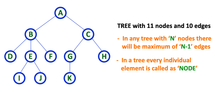
In tree data structure, every individual element is called as Node. Node in a tree data structure stores the actual data of that particular element and link to next element in hierarchical structure.
In a tree data structure, if we have N number of nodes then we can have a maximum of N-1 number of links.
- Array Method
- Linked List Method
- Introduction to Tree in Data Structures
- The Necessity for a Tree in Data Structures
- Tree Node
- Tree Terminologies
- Root
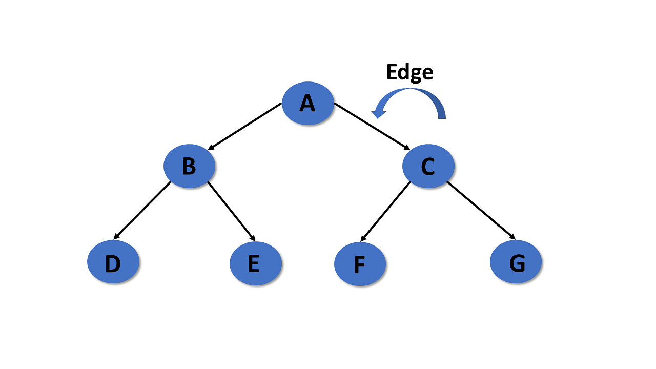
- Edge
- Parent
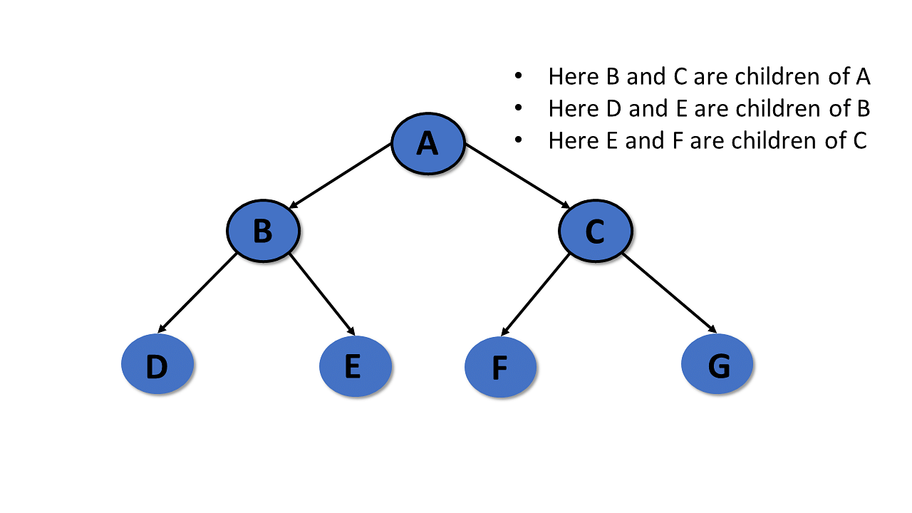
- Child
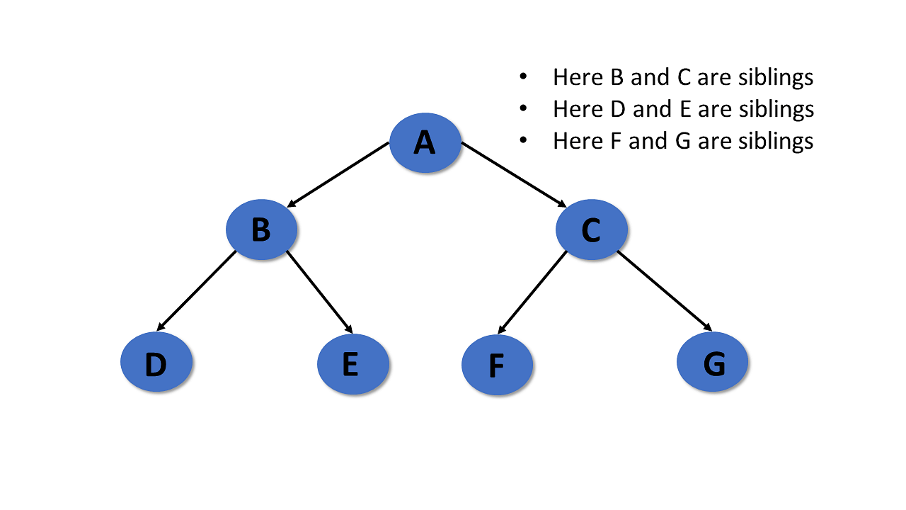
- Siblings
- Leaf
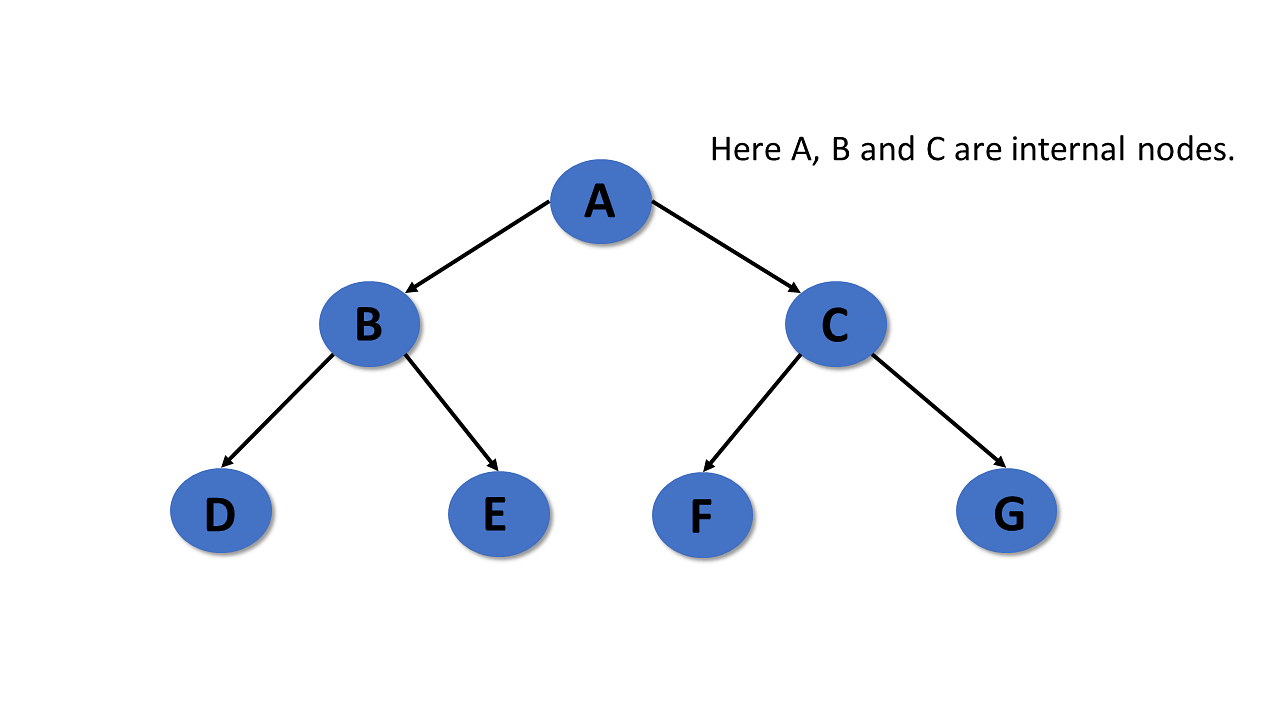
- Internal nodes
- Degree
- Level
- Height
- Depth
- Path
- Subtree
- Types of Tree in Data Structures
- General Tree
- Properties
- Binary Tree
- Properties
- Binary Search Tree
- Properties
- AVL Tree
- Properties
- Red-Black Tree
- Properties
- Splay Tree
- Properties
- Treap Tree
- Properties
- Tree Traversal
- In-Order Traversal
- Pre-Order Traversal
- Post-Order Traversal
- Application of Tree in Data Structures
- Next Step
- С++
- C
- Вывод:
- Sub Tree
- Complete Binary Tree
- Similar Binary Tree
- Complete Binary Tree
- Threaded Binary Tree
- Copy of Tree Data Structure
- Binary Tree Representation Using Linked List Representation:
- Operation On Binary Tree
- Traversing of Binary tree data structure:
- Inorder Traversal
- Balanced Binary Tree
- 1. Height Balanced Trees
- 2. Weight Balanced Trees
- Left Skewed Binary Tree
- AVL Tree Data structure
- Root
- Siblings
- Path
- Types of Binary Tree
- Example
- Expression Tree Data structure
- Internal Nodes
- Height
- Important Terms
- Basic Terminologies
- Parent
- Leaf
- Almost Complete Binary Tree
- Right Skewed Binary Tree
- 7. Balanced Binary Tree
- Edge
- Types of Trees
- General Trees
- Binary Trees
- Binary Search Trees
- Balanced Binary Search Trees
- Level
- Depth
- Degree
- Postorder Traversal
- Child
- Full Binary Tree
- 2. Perfect Binary Tree
- Recommended Post
Array Method
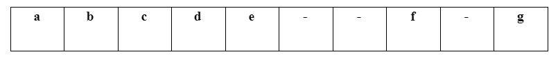
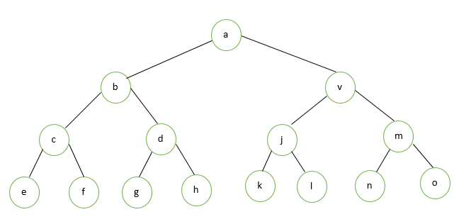
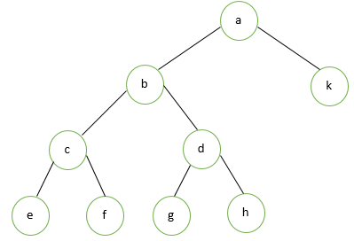
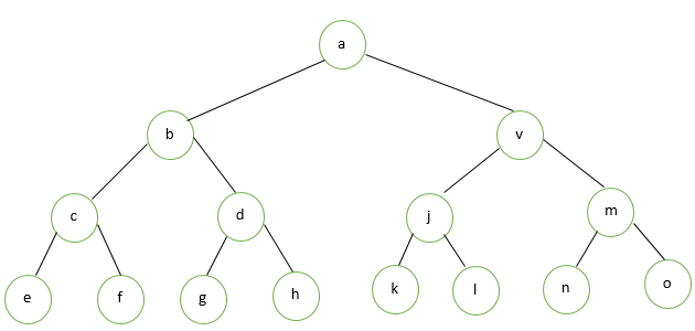
In this method, a binary tree is represented using a single-dimensional array. So for this purpose, the root node will be considered at zero index position. Based on the position of the parent, the left and right child will be calculated. So, the left child will be placed at ‘2n+1’ and the right child will place at ‘2n+2’. Here n is the position of parent.
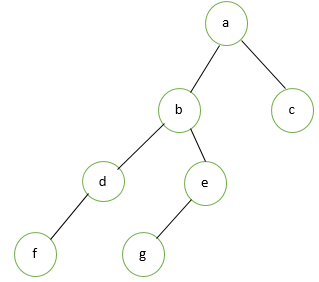
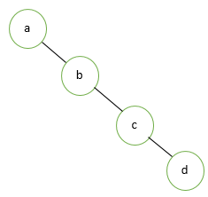
In this tree, ‘a’ is the root node so it will be placed at zero index in an array.
For the index position of left child ‘b’ :

For the index location of the right child ‘c’:

For the index location of the left child of ‘d’:

For the index location of the right child of ‘e’:

For the index location of the left child of ‘f’:

For the index location of the left child of ‘g’:

The tree is a non-linear data structure. This structure is mainly used to represent data containing a hierarchal relationship between elements (For example) record, family relationship, and table contents. The earth structure is a good example of a tree.

All data elements are in trees are called nodes. The node, which does not have its preceding nodes, is called ROOT node and it is considered at level number one. If a tree has ROOT node N and S1 and S2 left and right successor then N is called parent or father and S1 is called left child and S2 is called the right child. S1 and S2 are called brothers or siblings. The node on the same level is called “NODE OF THE SAME GENERATION”.
Linked List Method
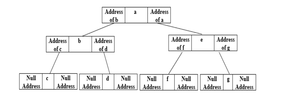
In this, a double-linked list will be used to represent every single node of the binary tree. In a doubly-linked list, there will be three fields i.e. address of the left child, root and address of right child fields.

Let us consider an example in which a binary tree has been taken with two children on each node. ’a’ is the root node in this tree. Every node has a left and right pointer. The left pointer will point towards the left child of the node and the right pointer will point towards the right node. The left and child addresses for leaf nodes will be assigned as ‘Null Address’.
Binary Tree Traversals
A binary tree consists of different nodes. So there are three methods to traverse a tree:
Node: It is an element of a tree.
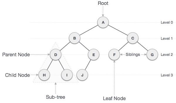
Root: It is the starting node of a tree. It is the top most element that has no parent element.
Parent Node: It is the node that has branches from top to bottom. It is the immediate predecessor of any node.
Child Node: It is the node that has a node from bottom to top. It is the instantaneous successor of any node.
Level: Each step in a tree is level.
Leaf Node: It is the node having no child.
Non-Leaf Node: It is the node having at least one child.
Edge: It is the link between two nodes.
Sibling: It is the child node with the same parents.
Internal Nodes: These are the nodes that have child nodes.
Degree: It is the largest number of child nodes.
Path: It is a sequence of nodes along with the boundaries of a tree.
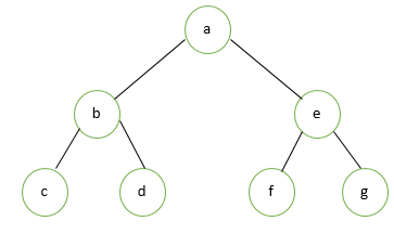
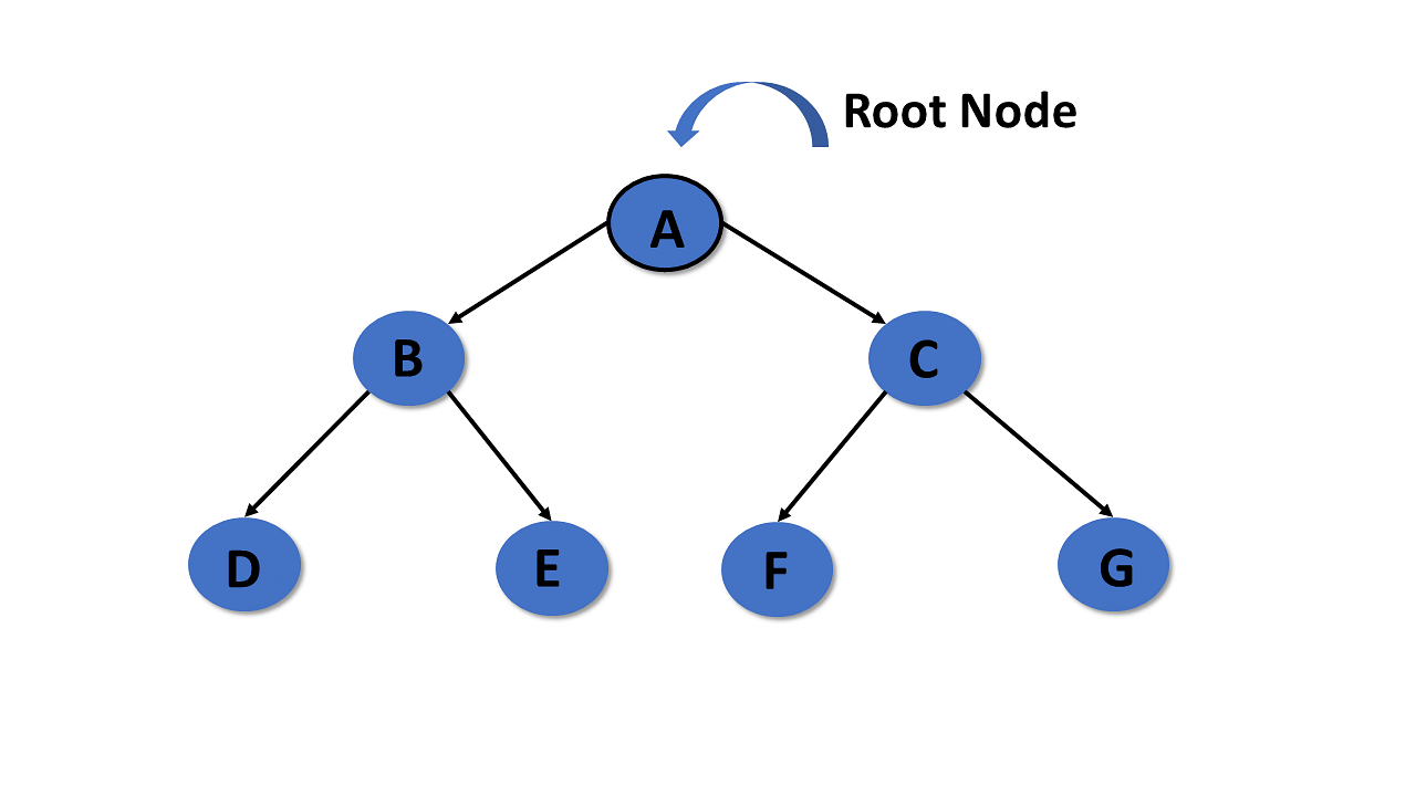
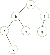
In a binary tree, every node in a tree should have a maximum of two children. It means that a tree can constitute either 0, 1, or 2 nodes. Let’s consider a tree shown below. In this figure, node ‘a’ has two children(b and f). Similarly, node b has also two children (d and e) and the same for node f. And node ‘f ’ has also two children (g and h) Each node has a maximum of two children. A binary tree usually consists of three nodes:

You must have observed the different parts of trees, from your childhood. A tree has roots, stems, branches, and leaves. And each leaf in a tree linked through roots via a unique path. Hence, similarly, a tree in data structures possesses hierarchical relationships, e.g. family tree, Document Object Model (DOM) in HTML, etc.
Introduction to Tree in Data Structures
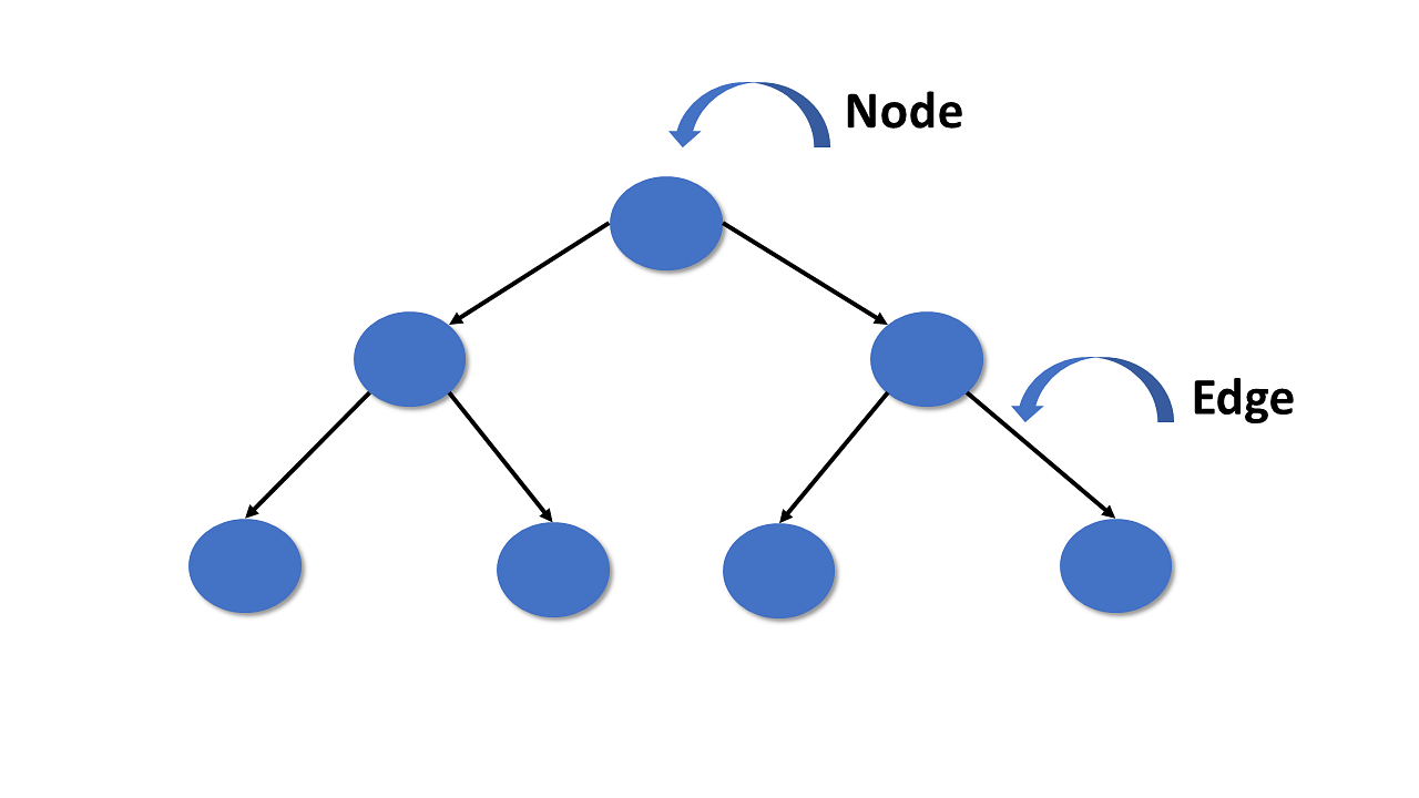
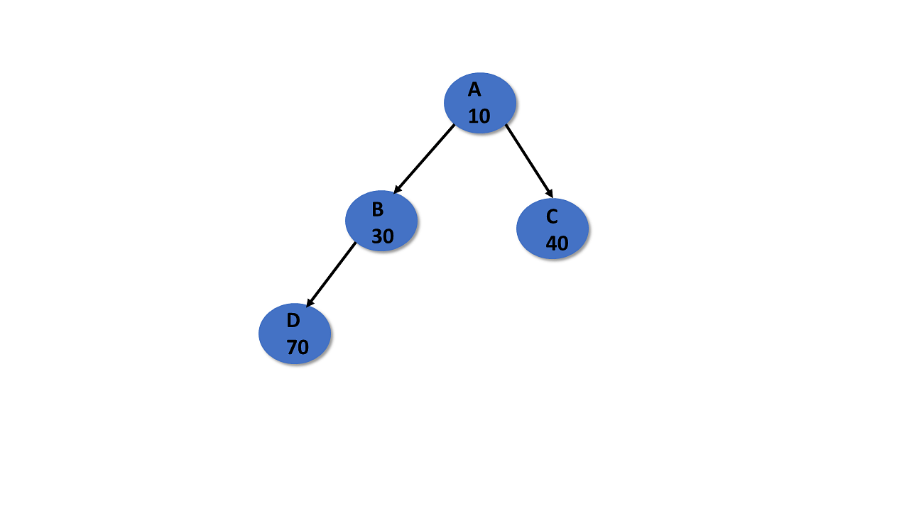
The tree is a nonlinear hierarchical data structure and comprises a collection of entities known as nodes. It connects each node in the tree data structure using «edges”, both directed and undirected.
The image below represents the tree data structure. The blue-colored circles depict the nodes of the tree and the black lines connecting each node with another are called edges.
You will understand the parts of trees better, in the terminologies section.
After learning the introduction to a tree in data structures, you will see why you need a tree in data structures.
The Necessity for a Tree in Data Structures
Other data structures like arrays, linked-list, stacks, and queues are linear data structures, and all these data structures store data in sequential order. Time complexity increases with increasing data size to perform operations like insertion and deletion on these linear data structures. But it is not acceptable for today’s world of computation.
The non-linear structure of trees enhances the data storing, data accessing, and manipulation processes by employing advanced control methods traversal through it. You will learn about tree traversal in the upcoming section.
But before that, understand the tree terminologies.
Tree Node
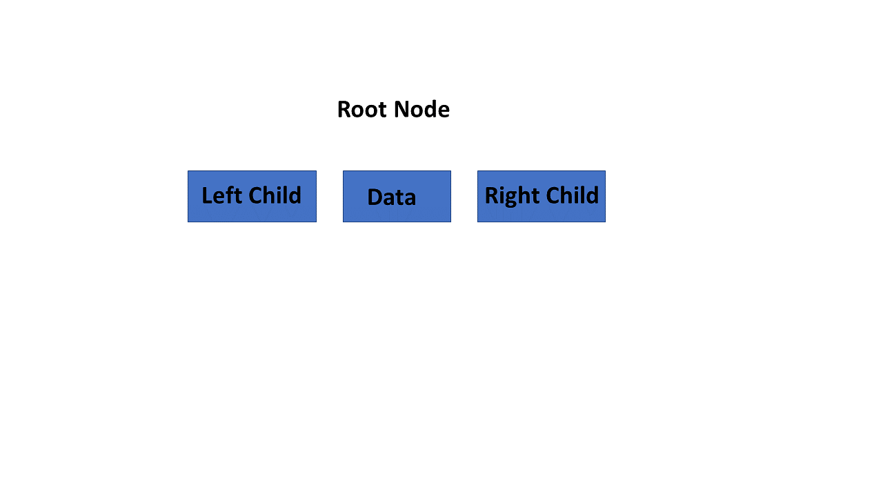
A node is a structure that contains a key or value and pointers in its child node in the tree data structure.
struct node *leftchild;
struct node *rightchild;
Continuing with this tutorial, you will see some key terminologies of the tree in data structures.
Tree Terminologies
Root
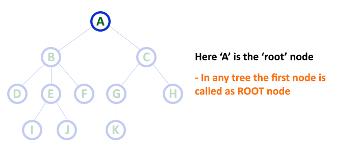
- In a tree data structure, the root is the first node of the tree. The root node is the initial node of the tree in data structures.
- In the tree data structure, there must be only one root node.
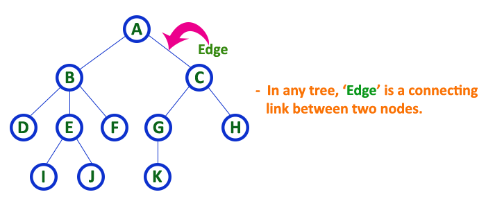
Edge
- In a tree in data structures, the connecting link of any two nodes is called the edge of the tree data structure.
- In the tree data structure, N number of nodes connecting with N -1 number of edges.
Parent
In the tree in data structures, the node that is the predecessor of any node is known as a parent node, or a node with a branch from itself to any other successive node is called the parent node.

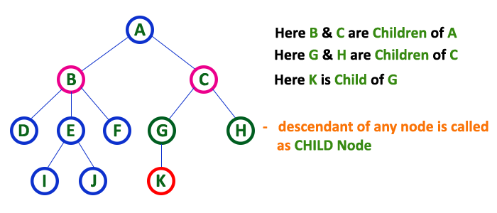
Child
- The node, a descendant of any node, is known as child nodes in data structures.
- In a tree, any number of parent nodes can have any number of child nodes.
- In a tree, every node except the root node is a child node.
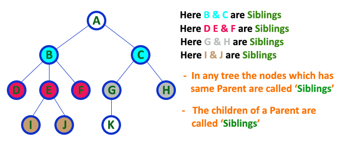
Siblings
In trees in the data structure, nodes that belong to the same parent are called siblings.
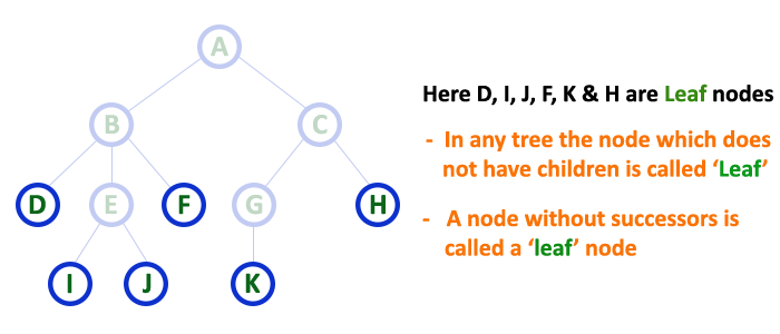
Leaf
- Trees in the data structure, the node with no child, is known as a leaf node.
- In trees, leaf nodes are also called external nodes or terminal nodes.

Internal nodes
- Trees in the data structure have at least one child node known as internal nodes.
- In trees, nodes other than leaf nodes are internal nodes.
- Sometimes root nodes are also called internal nodes if the tree has more than one node.
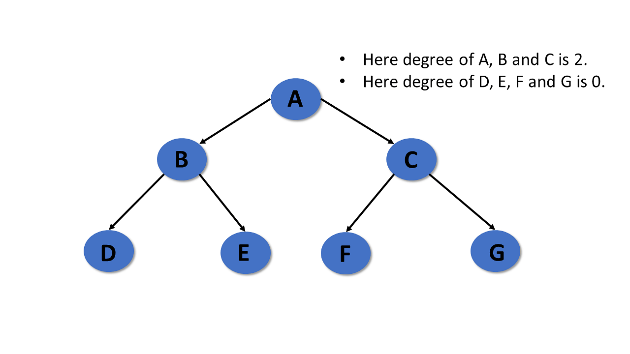
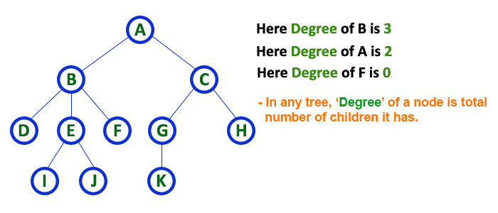
Degree
- In the tree data structure, the total number of children of a node is called the degree of the node.
- The highest degree of the node among all the nodes in a tree is called the Degree of Tree.
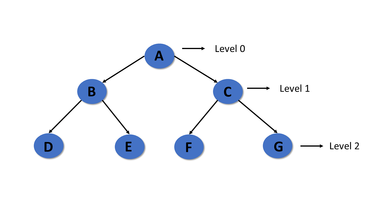
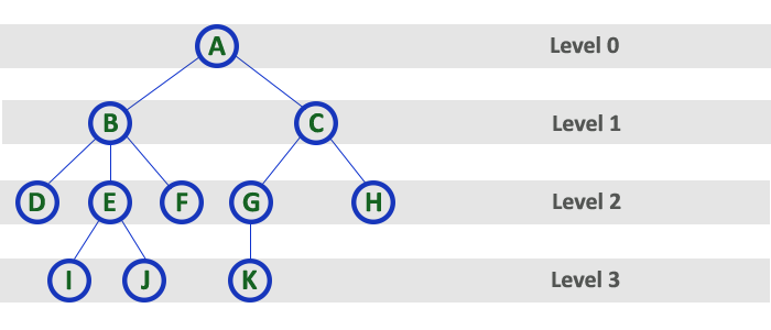
Level
In tree data structures, the root node is said to be at level 0, and the root node’s children are at level 1, and the children of that node at level 1 will be level 2, and so on.
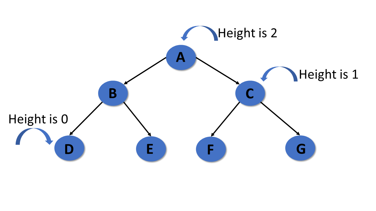
Height
- In a tree data structure, the number of edges from the leaf node to the particular node in the longest path is known as the height of that node.
- In the tree, the height of the root node is called «Height of Tree».
- The tree height of all leaf nodes is 0.
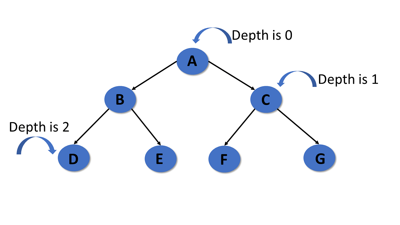
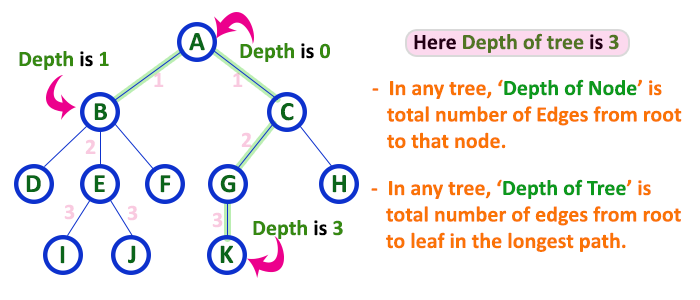
Depth
- In a tree, many edges from the root node to the particular node are called the depth of the tree.
- In the tree, the total number of edges from the root node to the leaf node in the longest path is known as «Depth of Tree».
- In the tree data structures, the depth of the root node is 0.
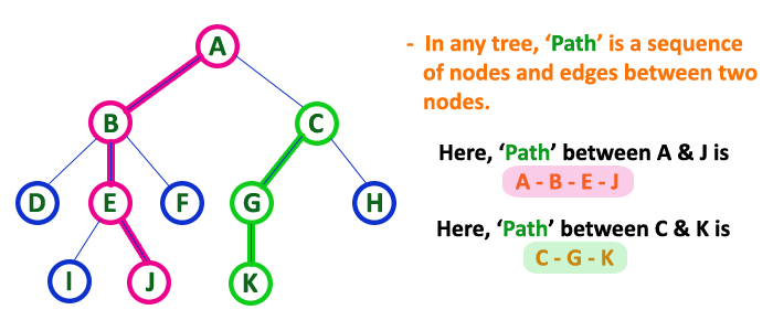
Path
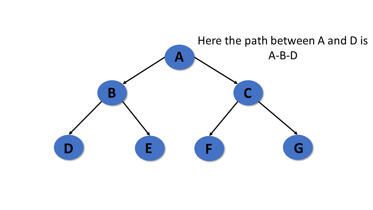
- In the tree in data structures, the sequence of nodes and edges from one node to another node is called the path between those two nodes.
- The length of a path is the total number of nodes in a path.zx
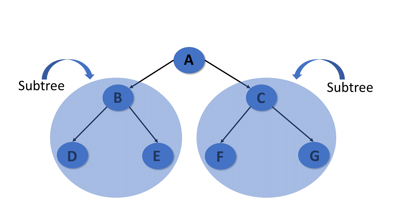
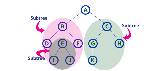
Subtree
In the tree in data structures, each child from a node shapes a sub-tree recursively and every child in the tree will form a sub-tree on its parent node.
Now you will look into the types of trees in data structures.
Types of Tree in Data Structures
Here are the different kinds of tree in data structures:
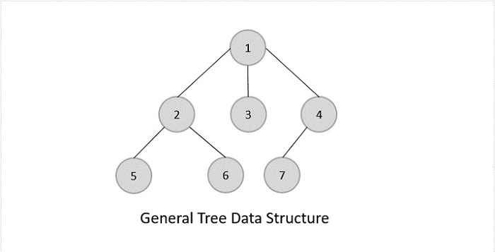
General Tree
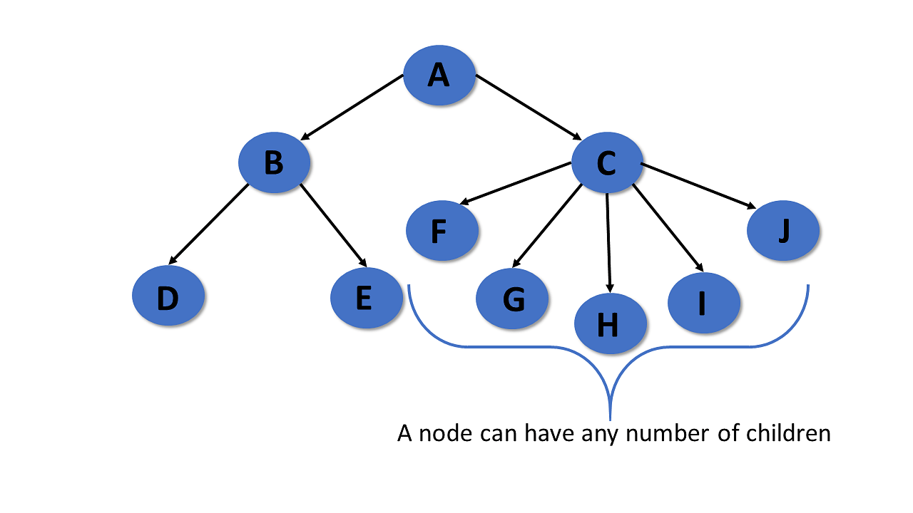
The general tree is the type of tree where there are no constraints on the hierarchical structure.
Properties
- The general tree follows all properties of the tree data structure.
- A node can have any number of nodes.
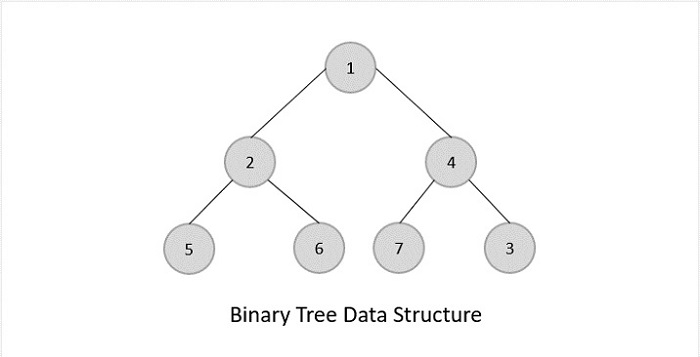
Binary Tree
Properties
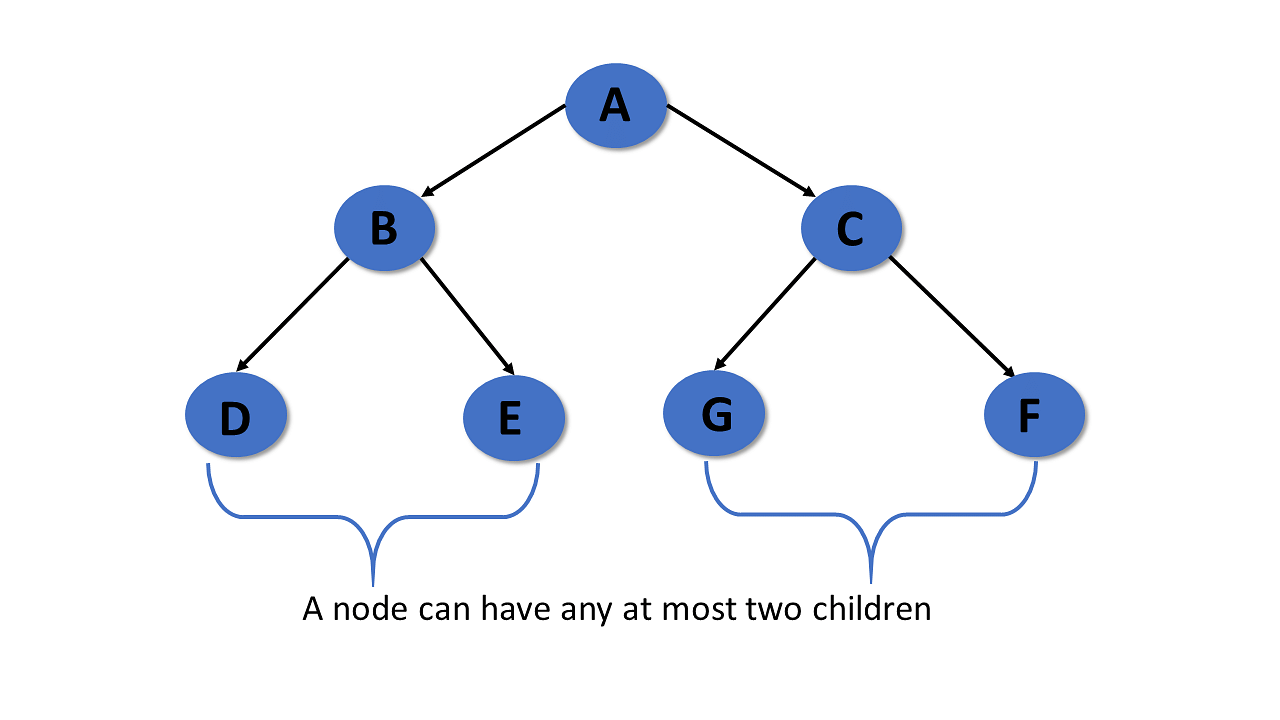
- Follows all properties of the tree data structure.
- Binary trees can have at most two child nodes.
- These two children are called the left child and the right child.
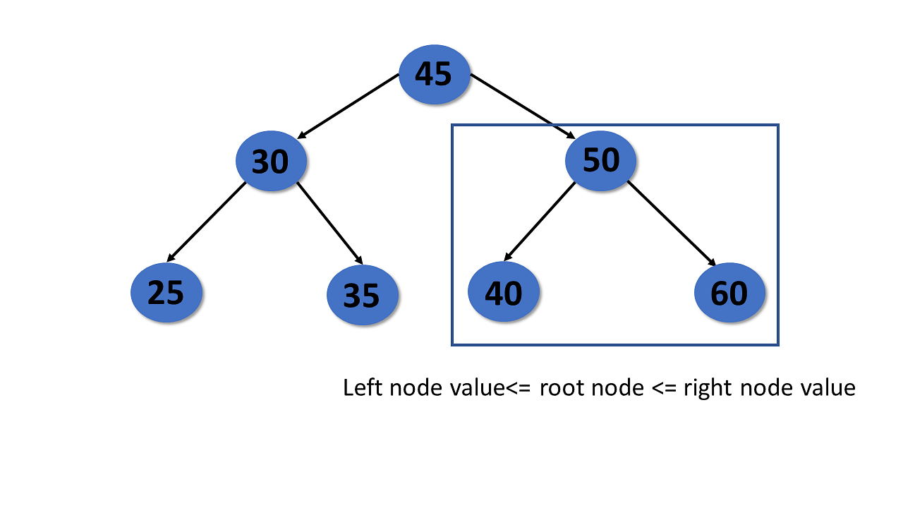
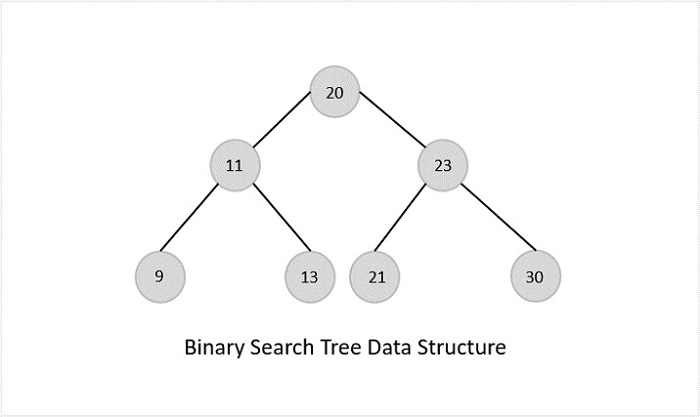
Binary Search Tree
A binary search tree is a type of tree that is a more constricted extension of a binary tree data structure.
Properties
- Follows all properties of the tree data structure.
- The binary search tree has a unique property known as the binary search property. This states that the value of a left child node of the tree should be less than or equal to the parent node value of the tree. And the value of the right child node should be greater than or equal to the parent value.
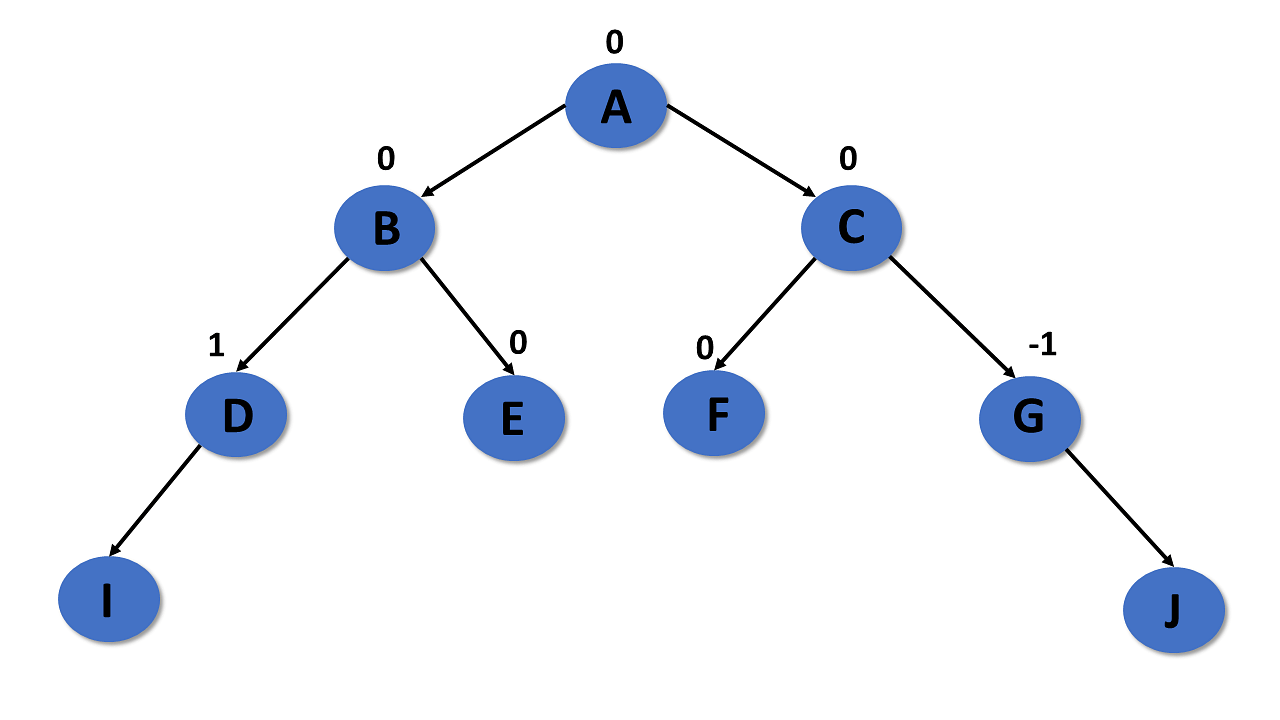
AVL Tree
An AVL tree is a type of tree that is a self-balancing binary search tree.
Properties
- Follows all properties of the tree data structure.
- Self-balancing.
- Each node stores a value called a balanced factor, which is the difference in the height of the left sub-tree and right sub-tree.
- All the nodes in the AVL tree must have a balance factor of -1, 0, and 1.
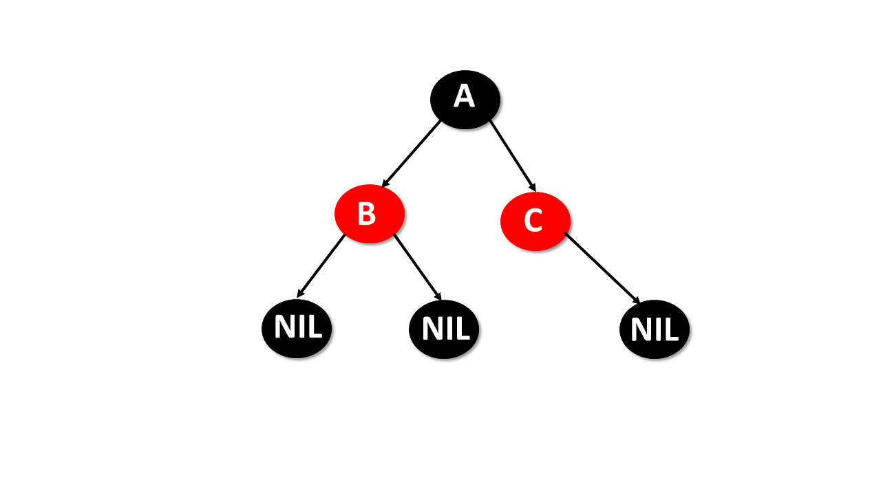
Red-Black Tree
- A red-black tree is a self-balancing binary search tree, where each node has either the color of red or black.
- The colors of the nodes are used to make sure that the tree remains approximately balanced during insertion and deletion.
Properties
- Follow all properties of binary tree data structure.
- Self-balancing.
- Each node is either red or black.
- The root and leaves nodes are black.
- If the node is red, then both children are black.
- Every path from a given node to any of its nodes must go through the same number of black nodes.
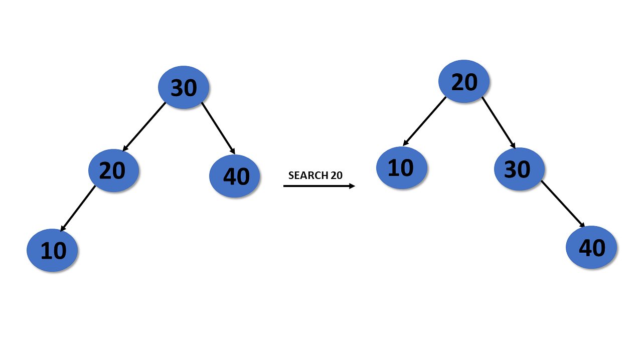
Splay Tree
A splay tree is a self-balancing binary search tree.
Properties
- Follows properties of binary tree data structure.
- Self-balancing.
- Recently accessed elements are quicker to access again.
After you perform operations such as insertion and deletion, the splay tree acts, which is called splaying. Here it rearranges the tree so that the particular elements are placed at the root of the tree.
Treap Tree
The Treap tree is made up of a tree, and the heap is a binary search tree.
Properties
- Each node has two values: a key and a priority.
- Follows a binary search tree property.
- Priority of the treap tree follows the heap property.
Tree Traversal
Traversal of the tree in data structures is a process of visiting each node and prints their value. There are three ways to traverse tree data structure.
- Pre-order Traversal
- In-Order Traversal
- Post-order Traversal
In-Order Traversal
In the in-order traversal, the left subtree is visited first, then the root, and later the right subtree.
Step 1- Recursively traverse the left subtree
Step 2- Visit root node
Step 3- Recursively traverse right subtree

Pre-Order Traversal
In pre-order traversal, it visits the root node first, then the left subtree, and lastly right subtree.
Step 1- Visit root node
Step 2- Recursively traverse the left subtree
Step 3- Recursively traverse right subtree

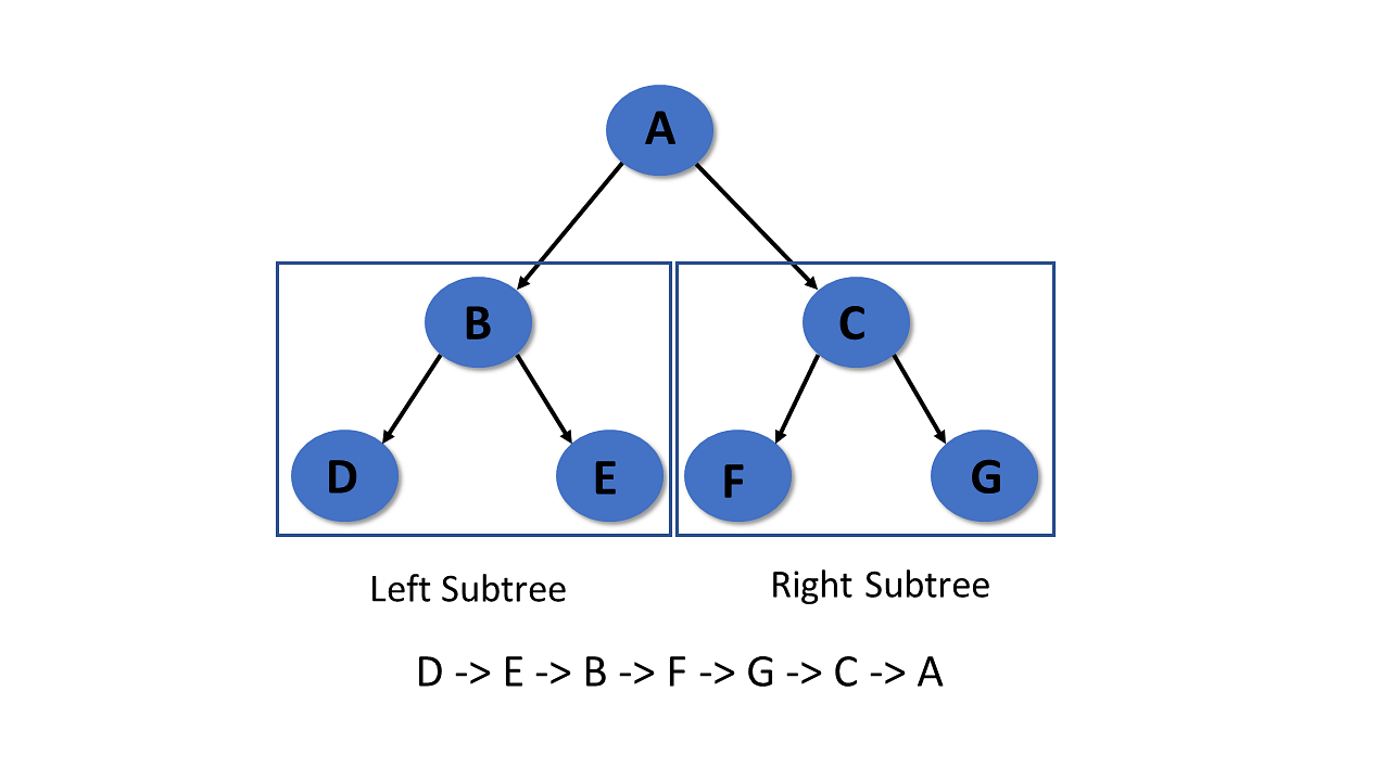
Post-Order Traversal
It visits the left subtree first in post-order traversal, then the right subtree, and finally the root node.
Step 1- Recursively traverse the left subtree
Step 2- Visit root node
Step 3- Recursively traverse right subtree
struct node* left;
struct node* right;
if (root == NULL) return;
printf(«%d ->», root->data);
if (root == NULL) return;
printf(«%d ->», root->data);
if (root == NULL) return;
printf(«%d ->», root->data);
struct node* newNode = malloc(sizeof(struct node));
newNode->data = item;
newNode->left = NULL;
newNode->right = NULL;
root->left = createNode(item);
root->right = createNode(item);
struct node* root = createNode(7);
Application of Tree in Data Structures
- Binary Search Tree (BST) is used to check whether elements present or not.
- Heap is a type of tree that is used to heap sort.
- Tries are the modified version of the tree used in modem routing to information of the router.
- The widespread database uses B-tree.
- Compilers use syntax trees to check every syntax of a program.
With this, you’ve come to the end of this tutorial about the tree in data structures.
Next Step
«Graphs in data structure» can be your next topic. As a tree data structure, the graph data structure is also a nonlinear data structure consisting of nodes and edges.
If you are interested in building a career in the field of software development, then feel free to explore Simplilearn’s Courses that will give you the work-ready software development training you need to succeed today. Are you perhaps looking for a more comprehensive training program in the most in-demand software development skills, tools, languages used today? If yes, our Post Graduate Program in Full Stack Development should prove to be just the right thing for your career. Explore the course and enroll soon.
If you have any questions regarding the “tree in data structures tutorial”, please let us know in the comment section below. Our experts will get back to you ASAP.
Перед прочтением этой статьи настоятельно рекомендуется ознакомиться с первой частью: Splay-дерево. Поиск
Как упоминалось в предыдущей статье, Splay-дерево — это самобалансирующаяся структура данных, в которой последний ключ, к которому осуществлялся доступ, всегда помещается в корень. Операция вставки аналогична вставке в бинарное дерево поиска с несколькими дополнительными шагами, цель которых убедиться, что вновь вставленный ключ становится новым корнем.
Ниже приведены различные случаи при вставке ключа k в Splay-дерево.
1) Корень равен NULL: мы просто создаем новый узел и возвращаем его как корневой.
2) Выполняем операцию Splay над заданный ключом k. Если k уже присутствует, он становится новым корнем. Если он отсутствует, то новым корневым узлом становится последний узел-лист, к которому был осуществлен доступ.
3) Если новый корневой ключ такой же, как k, ничего не делаем, поскольку k уже существует.
4) В противном случае выделяем память для нового узла и сравниваем корневой ключ с k.
4.a) Если k меньше корневого ключа, делаем корень правым дочерним элементом нового узла, копируем левый дочерний элемент корня в качестве левого дочернего элемента нового узла и делаем левый дочерний элемент корня равным NULL.
4.b) Если k больше корневого ключа, делаем корень левым дочерним элементом нового узла, копируем правый дочерний элемент корня в качестве правого дочернего элемента нового узла и делаем правый дочерний элемента корня равным NULL.
5) Возвращаем новый узел в качестве нового корня дерева.
100 [20] 25 / \ \ / \ 50 200 50 20 50 / insert(25) / \ insert(25) / \ 40 ======> 30 100 ========> 30 100 / 1. Splay(25) \ \ 2. insert 25 \ \ 30 40 200 40 200 / [20] С++
#include <bits/stdc++.h>
using namespace std;
// Узел АВЛ-дерева
class node
{ public: int key; node *left, *right;
};
/* Вспомогательная функция, которая выделяет
новый узел с заданным key и left и right, указывающими в NULL. */
node* newNode(int key)
{ node* Node = new node(); Node->key = key; Node->left = Node->right = NULL; return (Node);
}
// Служебная функция для разворота поддерева с корнем y вправо.
// Смотрите диаграмму, приведенную выше.
node *rightRotate(node *x)
{ node *y = x->left; x->left = y->right; y->right = x; return y;
}
// Служебная функция для разворота поддерева с корнем x влево
// Смотрите диаграмму, приведенную выше.
node *leftRotate(node *x)
{ node *y = x->right; x->right = y->left; y->left = x; return y;
}
// Эта функция поднимет ключ
// в корень, если он присутствует в дереве.
// Если такой ключ отсутствует в дереве, она
// поднимет в корень самый последний элемент,
// к которому был осуществлен доступ.
// Эта функция изменяет дерево
// и возвращает новый корень (root).
node *splay(node *root, int key)
{ // Базовые случаи: root равен NULL или // ключ находится в корне if (root == NULL || root->key == key) return root; // Ключ лежит в левом поддереве if (root->key > key) { // Ключа нет в дереве, мы закончили if (root->left == NULL) return root; // Zig-Zig (Левый-левый) if (root->left->key > key) { // Сначала рекурсивно поднимем // ключ в качестве корня left-left root->left->left = splay(root->left->left, key); // Первый разворот для root, // второй разворот выполняется после else root = rightRotate(root); } else if (root->left->key < key) // Zig-Zag (Left Right) { // Сначала рекурсивно поднимаем // ключ в качестве кореня left-right root->left->right = splay(root->left->right, key); // Выполняем первый разворот для root->left if (root->left->right != NULL) root->left = leftRotate(root->left); } // Выполняем второй разворот для корня return (root->left == NULL)? root: rightRotate(root); } else // Ключ находится в правом поддереве { // Ключа нет в дереве, мы закончили if (root->right == NULL) return root; // Zag-Zig (Правый-левый) if (root->right->key > key) { // Поднять ключ в качестве кореня right-left root->right->left = splay(root->right->left, key); // Выполняем первый поворот для root->right if (root->right->left != NULL) root->right = rightRotate(root->right); } else if (root->right->key < key)// Zag-Zag (Правый-правый) { // Поднимаем ключ в качестве корня // right-right и выполняем первый разворот root->right->right = splay(root->right->right, key); root = leftRotate(root); } // Выполняем второй разворот для root return (root->right == NULL)? root: leftRotate(root); }
}
// Функция для вставки нового ключа k в splay-дерево с заданным корнем
node *insert(node *root, int k)
{ // Простой случай: если дерево пусто if (root == NULL) return newNode(k); // Делаем ближайший узел-лист корнем root = splay(root, k); // Если ключ уже существует, то возвращаем его if (root->key == k) return root; // В противном случае выделяем память под новый узел node *newnode = newNode(k); // Если корневой ключ больше, делаем корень правым дочерним элементом нового узла, копируем левый дочерний элемент корня в качестве левого дочернего элемента нового узла if (root->key > k) { newnode->right = root; newnode->left = root->left; root->left = NULL; } // Если корневой ключ меньше, делаем корень левым дочерним элементом нового узла, копируем правый дочерний элемент корня в качестве правого дочернего элемента нового узла else { newnode->left = root; newnode->right = root->right; root->right = NULL; } return newnode; // новый узел становится новым корнем
}
// Служебная функция для вывода
// обхода в дерева ширину.
// Функция также выводит высоту каждого узла
void preOrder(node *root)
{ if (root != NULL) { cout<<root->key<<" "; preOrder(root->left); preOrder(root->right); }
}
/* Управляющий код */
int main()
{ node *root = newNode(100); root->left = newNode(50); root->right = newNode(200); root->left->left = newNode(40); root->left->left->left = newNode(30); root->left->left->left->left = newNode(20); root = insert(root, 25); cout<<"Preorder traversal of the modified Splay tree is \n"; preOrder(root); return 0;
}
// Этот код любезно предоставлен rathbhupendra
C
// Код позаимствован c http://algs4.cs.princeton.edu/33balanced/SplayBST.java.html
#include<stdio.h>
#include<stdlib.h>
// Узел АВЛ-дерева
struct node
{ int key; struct node *left, *right;
};
/* Вспомогательная функция, которая создает
новый узел с заданным key и left и right, указывающими в NULL. */
struct node* newNode(int key)
{ struct node* node = (struct node*)malloc(sizeof(struct node)); node->key = key; node->left = node->right = NULL; return (node);
}
// Служебная функция для разворота поддерева с корнем y вправо.
// Смотрите диаграмму, приведенную выше.
struct node *rightRotate(struct node *x)
{ struct node *y = x->left; x->left = y->right; y->right = x; return y;
}
// Служебная функция для разворота поддерева с корнем x влево
// Смотрите диаграмму, приведенную выше.
struct node *leftRotate(struct node *x)
{ struct node *y = x->right; x->right = y->left; y->left = x; return y;
}
// Эта функция поднимет ключ
// в корень, если он присутствует в дереве.
// Если такой ключ отсутствует в дереве, она
// поднимет в корень самый последний элемент,
// к которому был осуществлен доступ.
// Эта функция изменяет дерево
// и возвращает новый корень.
struct node *splay(struct node *root, int key)
{ // Базовые случаи: корень равен NULL или // ключ находится в корне if (root == NULL || root->key == key) return root; // Ключ лежит в левом поддереве if (root->key > key) { // Ключа нет в дереве, мы закончили if (root->left == NULL) return root; // Zig-Zig (Левый-левый) if (root->left->key > key) { // Сначала рекурсивно поднимем // ключ как корень left-left root->left->left = splay(root->left->left, key); // Первый разворот для корня, // второй разворот выполняется после else root = rightRotate(root); } else if (root->left->key < key) // Zig-Zag (Левый-правый) { // Сначала рекурсивно поднимаем // ключ как корень left-right root->left->right = splay(root->left->right, key); // Выполняем первый разворот для root->left if (root->left->right != NULL) root->left = leftRotate(root->left); } // Выполняем второй разворот для корня return (root->left == NULL)? root: rightRotate(root); } else // Ключ находится в правом поддереве { // Ключа нет в дереве, мы закончили if (root->right == NULL) return root; // Zag-Zig (Правый-левый) if (root->right->key > key) { //Поднимаем ключ в качестве корня right-left root->right->left = splay(root->right->left, key); // Выполняем первый поворот для root->right if (root->right->left != NULL) root->right = rightRotate(root->right); } else if (root->right->key < key)// Zag-Zag (Правый-правый) { // Поднимаем ключ в качестве корня // right-right и выполняем первый разворот root->right->right = splay(root->right->right, key); root = leftRotate(root); } //Выполняем второй разворот для корня return (root->right == NULL)? root: leftRotate(root); }
}
// Функция для вставки нового ключа k в splay-дерево с заданным корнем
struct node *insert(struct node *root, int k)
{ // Простой случай: если дерево пусто if (root == NULL) return newNode(k); // Делаем ближайший узел-лист корнем root = splay(root, k); // Если ключ уже существует, то возвращаем его if (root->key == k) return root; // В противном случае выделяем память под новый узел struct node *newnode = newNode(k); // Если корневой ключ больше, делаем корень правым дочерним элементом нового узла, копируем левый дочерний элемент корня в качестве левого дочернего элемента нового узла if (root->key > k) { newnode->right = root; newnode->left = root->left; root->left = NULL; } // Если корневой ключ меньше, делаем корень левым дочерним элементом нового узла, копируем правый дочерний элемент корня в качестве правого дочернего элемента нового узла else { newnode->left = root; newnode->right = root->right; root->right = NULL; } return newnode; // новый узел становится новым корнем
}
// Служебная функция для вывода
// обхода в дерева ширину.
// Функция также выводит высоту каждого узла
void preOrder(struct node *root)
{ if (root != NULL) { printf("%d ", root->key); preOrder(root->left); preOrder(root->right); }
}
/* Управляющий код для проверки приведенной выше функции */
int main()
{ struct node *root = newNode(100); root->left = newNode(50); root->right = newNode(200); root->left->left = newNode(40); root->left->left->left = newNode(30); root->left->left->left->left = newNode(20); root = insert(root, 25); printf("Preorder traversal of the modified Splay tree is \n"); preOrder(root); return 0;
}
Вывод:
Preorder traversal of the modified Splay tree is
25 20 50 30 40 100 200
Sub Tree
In a tree data structure, each child from a node forms a subtree recursively. Every child node will form a subtree on its parent node.
Complete Binary Tree
This is also called the “perfect binary tree”. In this, all levels are completely filled. And every node in each level must have two children and each level must comprising of 2N nodes. Where ‘N’ is the level number. And the last level has nodes as left as possible.

Properties of Complete Binary Tree
The maximum range of nodes in it are:

And x= Tree height.
2. The minimum range of nodes in it are:

3. Its maximum height for ‘n’ number of nodes is:

4. Its minimum height for ‘n’ number of nodes is:

Similar Binary Tree
Two binary trees T1 and T2 are said to be a similar binary trees if they have the same structure. In simple words, we say that if two trees have the same shape then they are called similar trees.

Complete Binary Tree
A tree is said to be a complete binary tree if it has exactly two nodes except the last node.

Threaded Binary Tree
Traversing a binary tree is a common operation and it would be helpful to find a more efficient method for implementing the traversal. Moreover, half of the entries in the Lchild and Rchild field will contain an NULL pointer. These fields may be used more efficiently by replacing the NULL entries with special pointers which point to nodes higher in the tree. Such types of special pointers are called threads and binary trees with such pointers are called threaded binary trees.
Copy of Tree Data Structure
Two binary tree T1 and T2 are said to be copy of each other if they have same structure and same contents.

Binary Tree Representation Using Linked List Representation:
The most popular and practical way of representing a binary tree is using a linked list (or pointers). In the linked list, every element is represented as a node. A node consists of three fields such as :
- Left Child (Lchild)
- Information of the Node (Info)
- Right Child (Rchild)
struct Tree
{ int information; struct Tree *Lchild; struct Tree *Rchild;
}
Operation On Binary Tree
- Create an empty binary tree
- Traversing a binary tree
- Inserting a Binary Tree
- Deleting a Node
- Searching for a Node
- Copying the mirror image of a tree
- Determine the total no: of Nodes
- Determine the total no: leaf Nodes
- Determine the total no: non-leaf Nodes
- Find the smallest element in a Node
- Finding the largest element
- Find the Height of the tree
- Finding the Father/Left Child/Right Child/Brother of an arbitrary node
Traversing of Binary tree data structure:
- Pre Order Traversing: –
- Visit the ROOT node.
- Traverse the LEFT subtree in pre-order.
- Traverse the RIGHT subtree in pre-order.
- In Order Traversing: –
- Traverse the LEFT subtree in pre-order.
- Visit the ROOT node.
- Traverse the RIGHT subtree in pre-order.
- Post Order Traversing: –
- Traverse the LEFT subtree in pre-order.
- Traverse the RIGHT subtree in pre-order.
- Visit the ROOT node.
[a +(b-c)] * [d –c) / (f + g –h)]
Pre order traversing:
* + a - b c / - d e - + f g hPost Order traversing:
a b c - + d e - f g + h - / *Inorder Traversal
Left Child >> Root Node >> Right Child
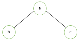
In the above tree, a root node is ‘a’ while left and right nodes are ‘b’ and ‘c’.Its inorder traversal will be:
Balanced Binary Tree
A balanced binary tree is one in which the largest path through the left subtree is the same length as the largest path of the right subtree, i.e., from root to leaf. Searching time is very less in balanced binary trees compared to unbalanced binary trees. i.e., balanced trees are used to maximize the efficiency of the operations on the tree.
There are two types of balanced trees :
- Height Balanced Trees
- Weight Balanced Trees
1. Height Balanced Trees
In height-balanced trees balancing the height is the important factor. There are two main approaches, which may be used to balance (or decrease) the depth of a binary tree :
- Insert a number of elements into a binary tree in the usual way, using the algorithm given in the previous section (i.e., Binary search Tree insertion). After inserting the elements, copy the tree into another binary tree in such a way that the tree is balanced. This method is efficient if the data(s) are continually added to the tree.
- Another popular algorithm for constructing a height-balanced binary tree is the AVL tree, which is discussed in the next section.
2. Weight Balanced Trees
A weight-balanced tree is a balanced binary tree in which an additional weight field is also there. The nodes of a weight-balanced tree contain four fields:
- Data Element
- Left Pointer
- Right Pointer
- A probability or weight field
The data element left and right pointer fields are save as that in any other tree node. The probability field is a specially added field for a weight-balanced tree. This field holds the probability of the node being accessed again, that is the number of times the node has been previously searched for.
Left Skewed Binary Tree
It consists of nodes consisting of only left children. It has only left subtree or only left children. It is the left side-dominated tree. All the right side children remain null.
Let us consider an example as shown below. In this, the root node is ‘a’ and the leaf node is ‘d’. While internal nodes are ‘b’ and ‘d’.

AVL Tree Data structure
This algorithm was developed in 1962 by two Russian Mathematicians, G.M. Adel’s son Vel’sky and E.M. Landis; here the tree is called AVL Tree. An AVL tree is a binary tree in which the left and right subtree of any node may differ in height by at most 1, and in which both the subtrees are themselves AVL Trees.
- A node is called left heavy if the largest path in its left subtree is one level larger than the largest path of its right subtree.
- A node is called right heavy if the largest path in its right subtree is one level larger than the largest path of its left subtree.
- The node is called balanced if the largest paths in both the right and left subtrees are equal.
Root
In a tree data structure, the first node is called as Root Node. Every tree must have a root node. We can say that the root node is the origin of the tree data structure. In any tree, there must be only one root node. We never have multiple root nodes in a tree.
Siblings
In a tree data structure, nodes which belong to same Parent are called as SIBLINGS. In simple words, the nodes with the same parent are called Sibling nodes.
Path
In a tree data structure, the sequence of Nodes and Edges from one node to another node is called as PATH between that two Nodes. Length of a Path is total number of nodes in that path. In below example the path A — B — E — J has length 4.
Types of Binary Tree
Full Binary Tree.
Perfect Binary Tree.
Almost Complete Binary Tree.
Complete Binary Tree.
Left Skewed Binary Tree.
Right Skewed Binary Tree
Balanced Binary Tree
Example
Expression Tree Data structure
An ordered tree may be used to represent a general expression, which is called an expression tree. Nodes in one expression tree contain operators and operands.
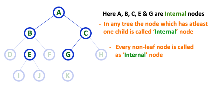
Internal Nodes
In a tree data structure, the node which has atleast one child is called as INTERNAL Node. In simple words, an internal node is a node with atleast one child.
In a tree data structure, nodes other than leaf nodes are called as Internal Nodes. The root node is also said to be Internal Node if the tree has more than one node.
Internal nodes are also called as ‘Non-Terminal‘ nodes.
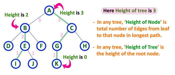
Height
In a tree data structure, the total number of edges from leaf node to a particular node in the longest path is called as HEIGHT of that Node. In a tree, height of the root node is said to be height of the tree. In a tree, height of all leaf nodes is ‘0’.
Important Terms
Path − Path refers to the sequence of nodes along the edges of a tree.
Root − The node at the top of the tree is called root. There is only one root per tree and one path from the root node to any node.
Parent − Any node except the root node has one edge upward to a node called parent.
Child − The node below a given node connected by its edge downward is called its child node.
Leaf − The node which does not have any child node is called the leaf node.
Subtree − Subtree represents the descendants of a node.
Visiting − Visiting refers to checking the value of a node when control is on the node.
Traversing − Traversing means passing through nodes in a specific order.
Levels − Level of a node represents the generation of a node. If the root node is at level 0, then its next child node is at level 1, its grandchild is at level 2, and so on.
Keys − Key represents a value of a node based on which a search operation is to be carried out for a node.
Basic Terminologies
- The root is a specially designed node (or data items) in a tree. It is the first node in the hierarchical arrangement of the data items. Each data item in a tree is called a node. It specifies the data information and links (branches) to other data items.
- A node is a structure that may contain a value, a condition, or represent a separate data structure (which could be a tree of its own). Each node in a tree has zero or more child nodes, which are below it in the tree (by convention, trees are drawn growing downwards). A node that has a child is called the child’s parent node (or ancestor node, or superior). A node has at most one parent
- An internal node (also known as an inner node or branch node) is any node of a tree that has child nodes.
- Similarly, an external node (also known as an outer node, leaf node, or terminal node) is any node that does not have child nodes.
- The topmost node in a tree is called the root node. Being the topmost node, the root node will not have a parent. It is the node at which operations on the tree commonly begin (although some algorithms begin with the leaf nodes and work up ending at the root). All other nodes can be reached from it by following edges or links. (In the formal definition, each such path is also unique). In some trees, such as heaps, the root node has special properties. Every node in a tree can be seen as the root node of the subtree rooted at that node. A free tree is a tree that is not rooted.
- The height of a node is the length of the longest downward path to a leaf from that node. The height of the root is the height of the tree.
- The depth of a node is the length of the path to its root (i.e., its root path). This is commonly needed in the manipulation of the various self-balancing trees, AVL Trees in particular. Conventionally, the value −1 corresponds to a subtree with no nodes, whereas zero corresponds to a subtree with one node.
- A subtree of a tree T is a tree consisting of a node in T and all of its descendants in T. (This is different from the formal definition of subtree used in graph theory.) The subtree corresponding to the root node is the entire tree; the subtree corresponding to any other node is called a proper subtree (in analogy to the term proper subset).
A tree is said to be a binary tree if it has at most two nodes. In simple words, we say that a binary tree must have zero, one, or two nodes. A binary tree is a very important tree structure.

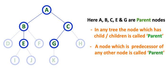
Parent
In a tree data structure, the node which is a predecessor of any node is called as PARENT NODE. In simple words, the node which has a branch from it to any other node is called a parent node. Parent node can also be defined as «The node which has child / children«.
Leaf
In a tree data structure, the node which does not have a child is called as LEAF Node. In simple words, a leaf is a node with no child.
In a tree data structure, the leaf nodes are also called as External Nodes. External node is also a node with no child. In a tree,
leaf node is also called as ‘Terminal‘ node.
Almost Complete Binary Tree
It is also named an “incomplete binary tree”. In this sort of binary tree, every single node must have two children in all levels apart from the last level but the first left child should be filled and then the right one.
Let us consider an example below. In this , there are a total five levels(0,1,2,3,4). In level 1, there are a total of 2 nodes in which each of the nodes has two children. Similarly, level 2 has 4 and level 3 has 8 nodes with their corresponding two children. Then we have two leaf nodes x and y at the end which are filled from left to right.

Right Skewed Binary Tree
In this type of binary tree, there exist nodes consisting of only the right children. It is vice versa of the left-skewed binary tree. It is a right-side-dominated tree. It contains no left child.
7. Balanced Binary Tree
In this, the height of the left subtree and right subtree of every single node might vary by one.
Binary Tree Representation
A binary tree can be represented by two methods.
Using Array Method
Using the Linked List Method
Edge
In a tree data structure, the connecting link between any two nodes is called as EDGE. In a tree with ‘N‘ number of nodes there will be a maximum of ‘N-1‘ number of edges.
Types of Trees
There are three types of trees −
Binary Search Trees
General Trees
General trees are unordered tree data structures where the root node has minimum 0 or maximum ‘n’ subtrees.
The General trees have no constraint placed on their hierarchy. The root node thus acts like the superset of all the other subtrees.
Binary Trees
Binary Trees are general trees in which the root node can only hold up to maximum 2 subtrees: left subtree and right subtree. Based on the number of children, binary trees are divided into three types.
Full Binary Tree
A full binary tree is a binary tree type where every node has either 0 or 2 child nodes.
Complete Binary Tree
A complete binary tree is a binary tree type where all the leaf nodes must be on the same level. However, root and internal nodes in a complete binary tree can either have 0, 1 or 2 child nodes.
Perfect Binary Tree
A perfect binary tree is a binary tree type where all the leaf nodes are on the same level and every node except leaf nodes have 2 children.
Binary Search Trees
Binary Search Trees possess all the properties of Binary Trees including some extra properties of their own, based on some constraints, making them more efficient than binary trees.
The data in the Binary Search Trees (BST) is always stored in such a way that the values in the left subtree are always less than the values in the root node and the values in the right subtree are always greater than the values in the root node, i.e. left subtree < root node ≤ right subtree.
Advantages of BST
Binary Search Trees are more efficient than Binary Trees since time complexity for performing various operations reduces.
Since the order of keys is based on just the parent node, searching operation becomes simpler.
The alignment of BST also favors Range Queries, which are executed to find values existing between two keys. This helps in the Database Management System.
Disadvantages of BST
The main disadvantage of Binary Search Trees is that if all elements in nodes are either greater than or lesser than the root node, the tree becomes skewed. Simply put, the tree becomes slanted to one side completely.
This skewness will make the tree a linked list rather than a BST, since the worst case time complexity for searching operation becomes O(n).
To overcome this issue of skewness in the Binary Search Trees, the concept of Balanced Binary Search Trees was introduced.
Balanced Binary Search Trees
Consider a Binary Search Tree with ‘m’ as the height of the left subtree and ‘n’ as the height of the right subtree. If the value of (m-n) is equal to 0,1 or -1, the tree is said to be a Balanced Binary Search Tree.
The trees are designed in a way that they self-balance once the height difference exceeds 1. Binary Search Trees use rotations as self-balancing algorithms. There are four different types of rotations: Left Left, Right Right, Left Right, Right Left.
There are various types of self-balancing binary search trees −
Red Black Trees
Priority Search Trees
Level
Depth
In a tree data structure, the total number of egdes from root node to a particular node is called as DEPTH of that Node. In a tree, the total number of edges from root node to a leaf node in the longest path is said to be Depth of the tree. In simple words, the highest depth of any leaf node in a tree is said to be depth of that tree. In a tree, depth of the root node is ‘0’.
Degree
In a tree data structure, the total number of children of a node is called as DEGREE of that Node. In simple words, the Degree of a node is total number of children it has. The highest degree of a node among all the nodes in a tree is called as ‘Degree of Tree‘
Postorder Traversal
Left Child >> Right Child >> Root Node
To understand its concept, we will consider the previous binary tree. Its postorder traversal will be:
For preorder traversal, we have:

For postorder traversal, we have:

Properties of Binary Tree
The maximum range of nodes in it is:

And x= Tree height
2. The minimum range of nodes in it is:

3. Its maximum height for ‘n’ number of nodes is:

4. Its maximum height tree for ‘n’ number of nodes is:

Application of Binary Tree
It is used to find duplicate nodes.
It is also used in sorting and in the traversal.
Its practical application is in an organization where binary trees are used to organize data in a sequence.
It is also used in machine learning, database tables, encryption and routing.
Child
In a tree data structure, the node which is descendant of any node is called as CHILD Node. In simple words, the node which has a link from its parent node is called as child node. In a tree, any parent node can have any number of child nodes. In a tree, all the nodes except root are child nodes.
Full Binary Tree
Properties of Full Binary Tree

And x= height of the full binary tree
2. Its minimum range of nodes is:

3. Its maximum height for ‘n’ nodes is:

4. Its minimum height for ‘n’ nodes is:

5. The range of leaf nodes for ‘n’ internal nodes is :

2. Perfect Binary Tree
In this type, all the internal nodes must have two children and the entire leaf nodes are at a similar level. This can be a full and complete binary tree as well.
To understand, let us consider an example shown below. This binary tree consists of three levels: internal nodes contain two child each and leaf nodes are also at an equal level.
Properties of Perfect Binary Tree
The leaf nodes for ‘x’ height in it are:

2. The range of internal nodes in it is:

And x= height of the tree.
3. The maximum range of nodes in it is:

4. The minimum range of nodes in it is:

Recommended Post
If you find any error then you can simply comment below on the tree data structure.
Thank you so much!
")


")