

Sumit_shah asked. 2021-12-06
I’m trying to apply for estimating azimuth angle of a sound source in a real-world scenario. I’m doing this by recording an audio file in a 2-element ULA and placing the sound source at a specific angle( say 20 degree azimuth, 0 degree elevation
Below is the code I’ve written
Here I used two mono-signals recorded separately using 2-different microphones(LEFT & RIGHT) in a ULA. From above program, I’m getting a perfect az = 20.0000 20.0000 as output.
My Questions: — I had approximated the angles of the sound sources to be around 20 degrees azimuth, So I don’t expect the sound source to be at exactly 20 degrees as evaluated by the algorithm. So it appears that the output is because of the collectPlaneWave function parameters. — Do I have to use collectPlaneWave function in my real-world audio already recorded at a specific source angle ? (I tried not using this, but azimuth angle given by algorithm was always zero.)
Could you please help me out with this ? Thanks.
Rootmusicestimator , phased , doa estimation , music algorithm

John Michell answered . 2023-07-03 22:40:09
In your example, you simulated the received signal at 20 degrees, that’s why the estimated result is 20 degree. In real life, if you already have the signal, then you don’t need to use . You just send the recorded signal in as two channels. This being said, RootMUSIC applies only to narrow band signals. So depends on your setting, it may or may not be the right algorithm for your task.
BTW, you should consider setting the propagation speed too. You are getting the matching result because the propagation speed is consistent among components. However, all of them are set to speed of light.
Not satisfied with the answer ?? ASK NOW
w = rootmusic(x,p)
estimates the frequency content in the input signal x and returns
w, a vector of frequencies in rad/sample. You can specify the signal
subspace dimension using the input argument p.
The extra threshold parameter in the second entry in p provides you
more flexibility and control in assigning the noise and signal subspaces.
You can place ‘corr’ anywhere after p.
Examples
Estimate the amplitudes for two sinusoids in noise. The separation between the sinusoids is less than the resolution of the periodogram, radians/sample. Use the autocorrelation matrix as the input to rootmusic.
Input Arguments
Input signal, specified as a vector or matrix. If x is a
vector, then it is treated as one observation of the signal. If x
is a matrix, each row of x represents a separate observation of the
signal. For example, each row is one output of an array of sensors, as in array
processing, such that x’*x is an estimate of the correlation
matrix.
For complex-valued input data x, pow and
w have the same length. For real-valued input data
x, the length of the corresponding power vector
pow is 0.5*length(w).
You can use the output of corrmtx to generate such an array x.
Complex Number Support: Yes
P —
Subspace dimension, specified as a real positive integer or a two-element vector. If
p is a real positive integer, then it is treated as the subspace
dimension. If p is a two-element vector, the second element of
p represents a threshold that is multiplied by , the smallest estimated eigenvalue of the signal’s correlation matrix.
Eigenvalues below the threshold are assigned to the noise subspace. In this case, specifies the maximum dimension of the signal subspace. The extra
threshold parameter in the second entry in p provides you more
flexibility and control in assigning the noise and signal subspaces.
Fs —
Output frequencies in rad/sample, returned as a vector. The length of the vector
w is the computed dimension of the signal subspace.
Pow — Signal power
Signal power, returned as a vector.
F — Output frequencies in Hz
If the input signal x is real, and an odd number of sinusoids is
specified by p, an error message is displayed:
Real signals require an even number p of complex sinusoids.
Algorithms
The multiple signal classification (MUSIC) algorithm used by rootmusic
is the same as that used by pmusic. The algorithm performs eigenspace
analysis of the signal’s correlation matrix in order to estimate the signal’s frequency
content.
The difference between pmusic and rootmusic
is:
rootmusic is most useful for frequency estimation of signals made up of
a sum of sinusoids embedded in additive white Gaussian noise.
Extended Capabilities
Usage notes and limitations:
Generated code might return outputs in a different sorted order compared to MATLAB®.
Version History
Introduced before R2006a
MUltiple SIgnal Classification (MUSIC)
is a high-resolution direction-finding algorithm based on the eigenvalue
decomposition of the sensor covariance matrix observed at an array.
MUSIC belongs to the family of subspace-based direction-finding algorithms.
Signal Model
The signal model relates the received sensor data to the signals
emitted by the source. Assume that there are D uncorrelated
or partially correlated signal sources, sd(t).
The sensor data, xm(t),
consists of the signals, as received at the array, together with noise, nm(t).
A sensor data snapshot is the sensor data vector received at the M elements
of an array at a single time t.
An important quantity in any subspace method is the sensor
covariance matrix,Rx,
derived from the received signal data. When the signals are uncorrelated
with the noise, the sensor covariance matrix has two components, the signal
covariance matrix and the noise covariance
matrix.
where Rs is
the source covariance matrix. The diagonal
elements of the source covariance matrix represent source power and
the off-diagonal elements represent source correlations.
For uncorrelated sources
or even partially correlated sources, Rs is
a positive-definite Hermitian matrix and has full rank, D,
equal to the number of sources.
The signal covariance matrix, ARsAH,
is an M-by-M matrix, also with
rank D < M.
An assumption of the MUSIC algorithm is that the noise powers
are equal at all sensors and uncorrelated between sensors. With this
assumption, the noise covariance matrix becomes an M-by-M diagonal
matrix with equal values along the diagonal.
Because the true sensor covariance matrix is not known, MUSIC
estimates the sensor covariance matrix, Rx,
from the sensor covariance matrix. The
sample sensor covariance matrix is an average of multiple snapshots
of the sensor data
where T is
the number of snapshots.
Signal and Noise Subspaces
Therefore the arrival
vectors are orthogonal to the null subspace.
When noise is added, the eigenvectors of the sensor covariance
matrix with noise present are the same as the noise-free sensor covariance
matrix. The eigenvalues increase by the noise power. Let vi be
one of the original noise-free signal space eigenvectors. Then
shows that the signal
space eigenvalues increase by σ02.
The null subspace eigenvectors are also eigenvectors of Rx.
Let ui be one of the null
eigenvectors. Then
with eigenvalues of σ02 instead
of zero. The null subspace becomes the noise subspace.
MUSIC works by searching for all arrival vectors that are orthogonal
to the noise subspace. To do the search, MUSIC constructs an arrival-angle-dependent
power expression, called the MUSIC pseudospectrum:
When an arrival vector
is orthogonal to the noise subspace, the peaks of the pseudospectrum
are infinite. In practice, because there is noise, and because the
true covariance matrix is estimated by the sampled covariance matrix,
the arrival vectors are never exactly orthogonal to the noise subspace.
Then, the angles at which PMUSIC has
finite peaks are the desired directions of arrival. Because the pseudospectrum
can have more peaks than there are sources, the algorithm requires
that you specify the number of sources, D, as a
parameter. Then the algorithm picks the D largest
peaks. For a uniform linear array (ULA), the search space is a one-dimensional
grid of broadside angles. For planar and 3D arrays, the search space
is a two-dimensional grid of azimuth and elevation angles.
Root-MUSIC
For a ULA, the denominator in the pseudospectrum is a polynomial
in ,
but can also be considered a polynomial in the complex plane. In this
cases, you can use root-finding methods to solve for the roots, zi.
These roots do not necessarily lie on the unit circle. However, Root-MUSIC
assumes that the D roots closest to the unit circle
correspond to the true source directions. Then you can compute the
source directions from the phase of the complex roots.
Spatial Smoothing of Correlated Sources
When some of the D source signals are correlated, Rs is
rank deficient, meaning that it has fewer than D nonzero
eigenvalues. Therefore, the number of zero eigenvalues of ARsAH exceeds
the number, M – D, of zero eigenvalues for
the uncorrelated source case. MUSIC performance degrades when signals
are correlated, as occurs in a multipath propagation environment.
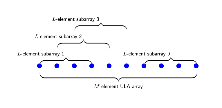
A way to compensate for correlation is to use spatial smoothing.
Spatial smoothing takes advantage of
the translation properties of a uniform array. Consider two correlated
signals arriving at an L-element ULA. The source
covariance matrix, Rs is
a singular 2-by-2 matrix. The arrival vector matrix is an L-by-2
matrix
for signals arriving
from the broadside angles φ1 and φ2.
The quantity k is the signal wave number. a(φ) represents
an arrival vector at the angle φ.
You can create a second array by translating the first array
along its axis by one element distance, d. The
arrival matrix for the second array is
where the arrival vectors
are equal to the original arrival vectors but multiplied by a direction-dependent
phase shift. When you translate the original array J –1 more
times, you get J copies of the array. If you form
a single array from all these copies, then the length of the single
array is M = L + (J – 1).
For the pth subarray, the source signal arrival
matrix is
The original arrival
vector matrix is postmultiplied by a diagonal phase matrix.
The last step is averaging the signal covariance matrices over
all J subarrays to form the averaged signal covariance
matrix, Ravgs.
The average signal covariance matrix depends on the smoothed source
covariance matrix, Rsmooth.
You can show that the
diagonal elements of the smoothed source covariance matrix are the
same as the diagonal elements of the original source covariance matrix.
However, the off-diagonal elements are reduced. The reduction
factor is the beam pattern of a J-element array.
In summary, you can reduce the degrading effect of source correlation
by forming subarrays and using the smoothed covariance matrix as input
to the MUSIC algorithm. Because of the beam pattern, larger angular
separation of sources leads to reduced correlation.
Spatial smoothing for linear arrays is easily extended to 2D
and 3D uniform arrays.
")


")