

Это руководство познакомит вас с тем, как найти корни многочлена с помощью функций roots() и solve() в MATLAB.

This tutorial will introduce how to find the roots of the polynomial using the roots() and solve() functions in MATLAB.
So far, we have seen that all the examples work in MATLAB as well as its GNU, alternatively called Octave. But for solving basic algebraic equations, both MATLAB and Octave are little different, so we will try to cover MATLAB and Octave in separate sections.
We will also discuss factorizing and simplification of algebraic expressions.
Polynomial calculations are very easy in Matlab®. Also, the calculation of roots of a polynomial can be very tough in calculus. Sometimes you can have a very long and complex polynomial to calculate its roots by hand. You can do this kind of stuff in Matlab® with the ‘roots()’ command very easily. Here, we explained the use of the ‘roots()’ command in Matlab® to find out the roots of polynomials, with a very basic example.

- Introduction to Matlab Root Finding
- Roots Function in Matlab with Examples
- Example #1
- Example #2
- Example #3
- Example #4
- Example #5
- Recommended Articles
- Introduction to Root Locus Matlab
- How to Do Root Locusmatlab?
- Examples of Root Locus Matlab
- Example 1
- Example 2
- Example #3
- Recommended Articles
- Introduction to Square Root in Matlab
- Working and Uses of Square Root in Matlab with Examples
- Example #1
- Example #2
- Example #3
- Conclusion
- Recommended Articles
- Usage of roots and solve in MATLAB
- Plotting graph using roots
- Roots of Scalar Functions
- Related Topics
- Get the Roots of the Polynomial Using the solve() Function in MATLAB
- Получите корни полинома с помощью функции solve() в MATLAB
- Solving System of Equations in Octave
- Solving Higher Order Equations in MATLAB
- Solving Quadratic Equations in MATLAB
- Expanding and Collecting Equations in Octave
- Factorization and Simplification of Algebraic Expressions
- Example
- Solving Basic Algebraic Equations in MATLAB
- Solving System of Equations in MATLAB
- Получите корни многочлена с помощью функции roots() в MATLAB
- Get the Roots of the Polynomial Using the roots() Function in MATLAB
- Solving Quadratic Equations in Octave
- Expanding and Collecting Equations in MATLAB
- Solving Higher Order Equations in Octave
- Solving Basic Algebraic Equations in Octave
- How To Use ‘roots()’ Command In Matlab®?
- Conclusion
Introduction to Matlab Root Finding
Roots of a polynomial are the values for which the polynomial equates to zero. So, if we have a polynomial in ‘x’, then the roots of this polynomial are the values that can be substituted in place of ‘x’ to make the polynomial equal to zero. Roots are also referred to as Zeros of the polynomial.
- If a polynomial has real roots, then the values of the roots are also the x-intercepts of the polynomial.
- If there are no real roots, the polynomial will not cut the x-axis at any point.
In MATLAB we use ‘roots’ function for finding the roots of a polynomial.
R = roots (Poly)
- R = roots (Poly) is used to find the roots of the input polynomial
- The input polynomial is passed as an argument in the form of a column vector
- For a polynomial of degree ‘p’, this column vector contains ‘p+1’ coefficients of the polynomial
Roots Function in Matlab with Examples
Let us now understand the code of roots functions in MATLAB using different examples:
Example #1
- Let our input polynomial be x^2 – x – 6
- Initialize the input polynomial in the form a column vector
- Passthiscolumn vector as an argument to the root function
R = roots(Poly)
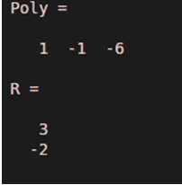
As we can see in the output, roots of the input polynomial x^2 – x -6 are 3, -2, which are the same as expected by us.
Example #2
- Let our input polynomial be x^3 –5x^2 + 2x+8
- Initialize the input polynomial in the form a column vector
- Pass this column vector as an argument to the root function
R = roots(Poly)
As we can see in the output, roots of the input polynomial x^3 – 5x^2 +2x +8 are 4, 2, -1, which are the same as expected by us.
Example #3
In the above 2 examples, we had polynomials with real roots. Let us now take some examples where polynomials have non-real roots.
- Let our input polynomial be x^5+2x^2 + x-2
- Initialize the input polynomial in the form a column vector
- Pass this column vector as an argument to the root function
R = roots(Poly)
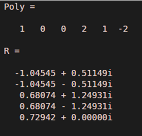
As we can see in the output, we have obtained complex roots for the input polynomial x^5 +2x^2 + x -2, as expected by us.
Example #4
- Let our input polynomial be x^2 + 1
- Initialize the input polynomial in the form a column vector
- Pass this column vector as an argument to the root function
R = roots(Poly)

As we can see in the output, we have obtained complex roots for the input polynomial x^2 + 1, as expected by us.
Example #5
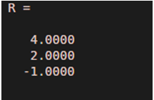
- Let our input polynomial be x^3 – 3x^2 – 4x + 12
- Initialize the input polynomial in the form a column vector
- Pass this column vector as an argument to the root function
R = roots(Poly)

As we can see in the output, the roots of the polynomial x^3 -3x^2 -4x 12 are -2, 3, 2
Recommended Articles
Updated March 8, 2023

Introduction to Root Locus Matlab
The W.R. Evans developed the root locus method. It is widely used in control engineering for the design and analysis of control systems. In this method, system poles are plotted against the value of a system parameter, especially the open-loop transfer function gain root locus analysis is a graphical method for examining how the roots of a system change with variation of a certain system parameter are typically used in control theory and stability theory. In this topic, we are going to learn about Root Locus Matlab.
The syntax for Root Locus Matlab is as shown below:-
How to Do Root Locusmatlab?
In a Matlab for a root locus, rlocus inbuilt function is available. For using these inbuilt rlocus function, we need to create one transfer function on a Matlab; for that, we can use a tf inbuilt function which can be available on Matlab.
Let us see how we used these function to display the root locus. For that, first, we need to create one transfer function. For creating a transfer function, we need to know the coefficients of the numerator and denominator of that transfer function
TF1 = tf (Num3 , Den3)
In a first way, we can take two variables to store the numerator and denominator coefficients and then we just pass those two variables on tf function and that a comma separates two variables.
Then use rlocus function in brackets the variable which is assigned for the transfer function.
Examples of Root Locus Matlab
Example 1
Let us consider one example,
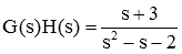
In this example, we take one transfer function for that we create two variables, ‘num1’ and ‘den1’, respectively. The variable ‘num1’ contains the coefficients of the numerator of the transfer function, and variable ‘den1’ stores the coefficients of the denominator of the transfer function. The tf function generates a transfer function for given coefficients of ‘num1’ and ‘den1’ variables on Matlab. Then using two variables of transfer function ‘num1’ and ‘den1’, we can display the transfer function and stored it in variable ‘TF1’.Then use the ‘rlocus’ function in brackets the variable which is assigned for transfer function ‘TF1’.
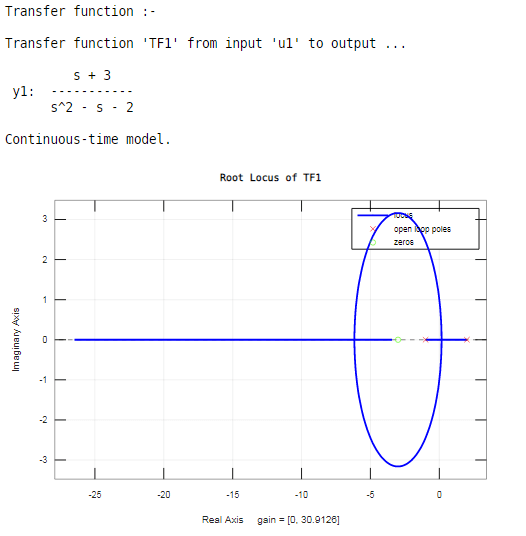
As shown in the resultant rot locus, it can show poles and zeros. For locating poles, the ‘×’ sign is used, and for zeros, the ‘o’ sign is used on a root locus.
Root locus exists on the real axis between:
2 and -1
-3 and negative infinity
Example 2
Let us see one more example related to root locus Matlab,

Example #3
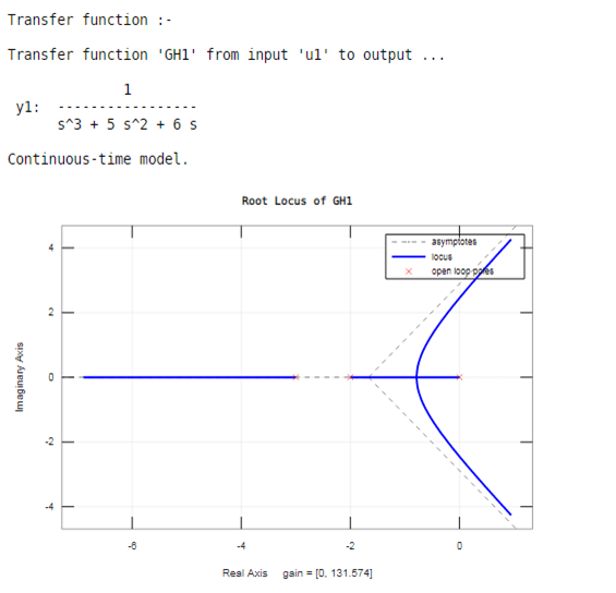
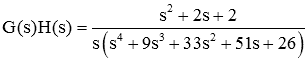
Let us consider another one example,
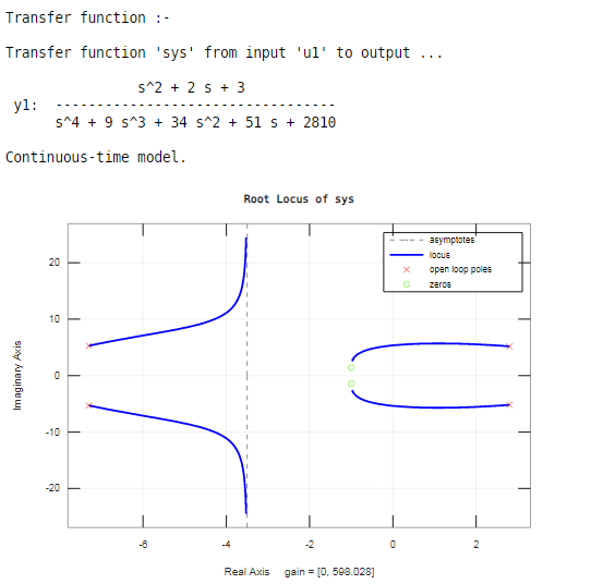
In this example, we have five poles and two zeros. The poles are shown by ‘×’, and the zeros are shown by ‘o’ on a root locus.
Root locus exists on the real axis between:
0 and -1
-2 and negative infinity
Recommended Articles
Updated March 24, 2023
Introduction to Square Root in Matlab
Square root is defined as taking the root of any square of a single element, a matrix or an array. Square root of a number can be positive or negative as a square of a positive number is positive and the square of a negative number is also positive. It is denoted by √ the symbol. Square root is simply the inverse method of squaring. If a^2 is the square integer, then a is defined as the square root of that number.
For example, 16 is a perfect square number and its square root can be 4 or -4. There are many methods that are used in mathematics to find the square root of a number.
Working and Uses of Square Root in Matlab with Examples
Matlab performs all mathematical functions, so there are also methods to find the square root of a number. In Matlab, we use the sqrt () function to find the square root of a number or each element defined in an array. The input arguments that are used in the function can be scalar, vector, array or multi-dimensional array. They can also be positive, negative or complex in nature. If the input is complex or negative in nature, then it results in a complex number.
Y = sqrt(x)
Example #1
Y = -3:3
So, the input is in the form of 1*7.
-3 -2 -1 0 1 2 3
(0.0000 + 1.7320i) (0.0000 + 1.4142i) (0.0000 + 1.0000i) (0.0000 + 0.0000i) (1.0000 + 0.0000i) (1.4142 + 0.0000i) (1.7320+0.0000i)
Example #2
Y = -5: -3
So the input is in the form of 1*4
-5 -4 -3
A = sqrt(Y)
(0.0000+2.2360i) (0.0000+2.0000i) (0.0000+1.7320i)
We know that is the input of an array is negative than it results in a complex number. In the above two examples, we see that the range consists of negative and positive numbers, so the output of it is a complex number. Some operations differ in Matlab as compared to IEEE standard like the square root of negative zero is 0 in Matlab while it is -0 in IEEE, square root of values less than zero results in a complex number in Matlab while the same is not available in IEEE.
If we want to find the square root of only positive integers in an array, then we can use realsqrt () function in Matlab. Unlike sqrt () function, it gives error messages when we pass input as a negative or complex number. So, if we want to view the result of a negative or complex number than it is preferable to use sqrt () function. The output size and input size should be the same if we use realsqrt ().
Example #3
Input is a 4*4 matrix named as A
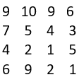
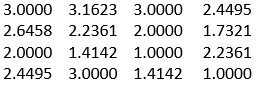
In the above example, it produces the square root of each element in a matrix. The input arguments can be a matrix, array, vector, scalar, or a multi-dimensional array and they should be positive and real integers. There are various properties of a square root in Matlab which should be noted:
The square root of any even number that is a perfect square should always be even.
For example: 16,36,64,100 etc.
Here 16, 36, 64 and 100 are all even numbers that are a perfect square and the square root of those numbers are 4,6,8 and 10 which are also even numbers.
The multiplication of square roots of the same number results in a positive integer while square roots of the number can also be multiplied and provide the output.
For example: √4 * √4 = 4
√3 * √2=√6
The square root of any odd number that is a perfect square should always be odd.
For example: 25,9,49,81
Here 25,9,47,81 are all perfect squares of odd numbers and the square root of those numbers are 5,3,7,9 which are also odd numbers. The unit digit of an element cannot be 3,2,8 or 7 to be a perfect square.
Conclusion
Square roots are widely used in Matlab for various business requirements. They are widely used in solving the solutions of any quadratic equations, machine learning topics like calculating standard deviation and variance. So, it is an essential feature in all the mathematical domains.
Recommended Articles
Both ways are shown in the script below:
Method 1 uses roots command and Method 2 uses symbolic and solve. You can verify that the function value at
is close to zero by entering
Using a Starting Point
Suppose you do not know two points at which the function values of
differ in sign.
Table of contents
Usage of roots and solve in MATLAB
I have an equation which goes like this:

Here a, b, c, d, e, f, g, h are constants. I want to vary k from say .6 to 10 with 0.1 interval and to find w. There are 2 ways to do this in MATLAB.
Another way is that defining symbolic functions and then executing the program. When you are using the this method, you may not need simplify the expression any further, you can just put it in first form itself (Method 2).
Both ways are shown in the script below:
%%% defining values
clear; clc;
a=0.1500;
b=0.20;
c=0.52;
d=0.5;
e=6;
f=30;
g=18;
h=2;
%% Method 1: varying k using roots
tic
i=0;
for k=.6:.1:10 i=i+1; t8=a; t7=0; t6=-(1+e+a*(c+g))*(k^2) ; t5=0; t4=(k^2*(b+f+(c*e+g)*k^2)-a*(d+h-c*g*k^4)); t3=0; t2=k^2*(d*(e+a*g)+h+a*c*h-(c*f+b*g)*k^2); t1=0; t0=(a*d*h)-(d*f+b*h)*k^2; q=[t8 t7 t6 t5 t4 t3 t2 t1 t0]; r(i,:)=roots(q);
end
krho1(:,1)=.6:.1:10;
r_real=real(r);
r_img=imag(r);
dat1=[krho1 r_real(:,1) r_real(:,2) r_real(:,3) r_real(:,4) r_real(:,5) r_real(:,6) r_real(:,7) r_real(:,8)];
fnameout=('stack_using_roots.dat');
fid1=fopen(fnameout,'w+');
fprintf(fid1,'krho\t RR1\t RR2\t RR3\t RR4\t RR5\t RR6\t RR7\t RR8\t \r');
fprintf(fid1,'%6.4f %7.10f %7.10f %7.10f %7.10f %7.10f %7.10f %7.10f %7.10f \n',dat1');
fclose(fid1);
plot(krho1, r_real(:,1),krho1, r_real(:,2),krho1, r_real(:,3),krho1, r_real(:,4),krho1, r_real(:,5),krho1, r_real(:,6),krho1, r_real(:,7),krho1, r_real(:,8))
toc
%% Method 2: varying k using solve
tic
syms w k
i=0;
for k=.6:.1:10 i=i+1; first=a/k^2; second=(w^2-b)/(w^4-k^2*c*w^2-d) ; third=(e*w^2-f)/(w^4-k^2*g*w^2-h); n(i,:)=double(solve(first-second-third, w));
end
krho1(:,1)=.6:.1:10;
r_real=real(n);
r_img=imag(n);
dat1=[krho1 r_real(:,1) r_real(:,2) r_real(:,3) r_real(:,4) r_real(:,5) r_real(:,6) r_real(:,7) r_real(:,8)];
fnameout=('stack_using_solve.dat');
fid1=fopen(fnameout,'w+');
fprintf(fid1,'krho\t RR1\t RR2\t RR3\t RR4\t RR5\t RR6\t RR7\t RR8\t \r');
fprintf(fid1,'%6.4f %7.10f %7.10f %7.10f %7.10f %7.10f %7.10f %7.10f %7.10f \n',dat1');
fclose(fid1);
figure;
plot(krho1, r_real(:,1),krho1, r_real(:,2),krho1, r_real(:,3),krho1, r_real(:,4),krho1, r_real(:,5),krho1, r_real(:,6),krho1, r_real(:,7),krho1, r_real(:,8))
toc- You can see that first section plots are coming in a short time, where the second one is taking a greater time. Is there any way to increase the speed?
- The plots of both the section seems very different, and you may be forced to believe that I have made mistakes while carrying out the calculation from
(a/k^2)-((w^2-b)/(w^4-k^2*c
w^2-d))-((e
w^2-f)/(w^4-k^2*g*w^2-h))
to
(something)w^8-(something else)w^6….-(something else again)w^0
. I can assure you that I have put it correctly. You can see what really happens, if you look for any particular value of krho in both the dat file (stack_using_roots and stack_using_solve). For, lets say, krho=3.6, the roots is the same in both the dat files, but the way in which it is ‘written’ is not in a proper way. That is why the plots looks awkward. In short, while using ‘roots’ command, the solutions are given in a orderd format, on the other hand while using ‘solve’, it is getting shifted randomly. What is really happening? Is there any way to get around this problem? I have ran the program with
i) syms w along with n(i,:)=double(solve(first-second-third==0, w));
ii) syms w k along with n(i,:)=double(solve(first-second-third==0, w));
iii) syms w k along with n(i,:)=double(solve(first-second-third, w));
In all these 3 cases, results seem to be same. Then what is the thing that we have to define as symbolic? And when do we use and do not use the expression ‘==0’?
- Are there any ways to increase the speed?
Several. Some trivial speed improvements would come from defining variables before the loop. The big bottleneck is
solve
. Unfortunately, there isn’t an obvious analytical solution to your problem without knowing
k
beforehand, so there’s no obvious way to pull
solve
outside the for loop.
- In short, while using ‘roots’ command, the solutions are given in a ordered format, on the other hand while using ‘solve’, it is getting shifted randomly. Why is that?
It is not
really
getting «shifted». Your function is symmetric about w = 0. So, for every root r there is another root at -r. Every time you call solve, it gives you the first, second, third then fourth roots, and then the same thing but this time the roots are
multiplied
by -1.
Sometimes solve chooses to take out -1 as a common factor. In these cases, it first gives you the roots multiplied by -1, then the positive roots. Why it sometimes takes out -1, sometimes doesn’t, I don’t know, but in your case (since you don’t care about the imaginary part) you can fix this by replacing
double(solve(first-second-third, w))
with
sort(real(double(solve(first-second-third, w))))
. The order of the roots won’t be the same as in Method 1, but you won’t get the weird switching behaviour.
- In all these 3 cases, results seem to be same. Then what is the thing that we have to define as symbolic? And when do we use and do not use the expression ‘==0’?
The reference page for
solve
dictates how the equation should be specified. If you scroll down to the section regarding the input variable
eqns
, it states
If any elements of
eqns
are symbolic expressions (without the right side), solve equates the element to 0.
This is why it makes no difference whether you write
first-second-third==0
or
first-second-third
as the first input to
solve
.
How to plot roots with a value used in the function?, I’m pretty new to matlab so sorry if this question seems trivial. My function is y = x^2 + bx -20. Im trying to find the roots for when b = 0 to 10 then plot the roots as a function of b.
Plotting graph using roots
The roots you have calculated are the x values where y = 0. Therefore to plot these on a graph you can use:
x = roots(p);
xaxis = -5:0.1:3;
y= xaxis.^3 + 5.5.*xaxis.^2 + 3.5.*xaxis — 10;
This shows the curve of the function over your specified interval and then plots circles at the roots you have obtained to highlight their location on the plot.
Usage of roots and solve in MATLAB, Every time you call solve, it gives you the first, second, third then fourth roots, and then the same thing but this time the roots are multiplied by -1. Sometimes solve chooses to take out -1 as a common factor. In these cases, it first gives you the roots multiplied by -1, then the positive roots.
Roots of Scalar Functions
Solving a Nonlinear Equation in One Variable
The
fzero
function attempts to find a root of one equation with one variable. You can call this function with either a one-element starting point or a two-element vector that designates a starting interval. If you give
fzero
a starting point
x0
,
fzero
first searches for an interval around this point where the function changes sign. If the interval is found,
fzero
returns a value near where the function changes sign. If no such interval is found,
fzero
returns
NaN
. Alternatively, if you know two points where the function value differs in sign, you can specify this starting interval using a two-element vector;
fzero
is guaranteed to narrow down the interval and return a value near a sign change.
x = -1:.01:2;
y = humps(x);
plot(x,y)
xlabel();
ylabel()
grid

Setting Options For
fzero
fzero
You can control several aspects of the
fzero
function by setting options. You set options using
optimset
. Options include:
Choosing the amount of display
fzero
generates — see Set Optimization Options, Using a Starting Interval, and Using a Starting Point.Choosing various tolerances that control how
fzero
determines it is at a root — see Set Optimization Options.Choosing a plot function for observing the progress of
fzero
towards a root — see Optimization Solver Plot Functions.Using a custom-programmed output function for observing the progress of
fzero
towards a root — see Optimization Solver Output Functions.
Using a Starting Interval
The graph of
humps
indicates that the function is negative at
x = -1
and positive at
x = 1
. You can confirm this by calculating
humps
at these two points.
To show the progress of
fzero
at each iteration, set the
Display
option to
iter
using the
optimset
function.
options = optimset(,);
a = fzero(@humps,[-1 1],options)
 Func-count x f(x) Procedure 2 -1 -5.13779 initial 3 -0.513876 -4.02235 interpolation 4 -0.513876 -4.02235 bisection 5 -0.473635 -3.83767 interpolation 6 -0.115287 0.414441 bisection 7 -0.115287 0.414441 interpolation 8 -0.132562 -0.0226907 interpolation 9 -0.131666 -0.0011492 interpolation 10 -0.131618 1.88371e-07 interpolation 11 -0.131618 -2.7935e-11 interpolation 12 -0.131618 8.88178e-16 interpolation 13 -0.131618 8.88178e-16 interpolation
Zero found in the interval [-1, 1]
Each value
x
represents the best endpoint so far. The
Procedure
column tells you whether each step of the algorithm uses bisection or interpolation.
You can verify that the function value at
a
is close to zero by entering
Using a Starting Point
Suppose you do not know two points at which the function values of
humps
differ in sign. In that case, you can choose a scalar
x0
as the starting point for
fzero
.
fzero
first searches for an interval around this point on which the function changes sign. If
fzero
finds such an interval, it proceeds with the algorithm described in the previous section. If no such interval is found,
fzero
returns
NaN
.
For example, set the starting point to
-0.2
, the
Display
option to
Iter
, and call
fzero
:
options = optimset(,);
a = fzero(@humps,-0.2,options)
Search for an interval around -0.2 containing a sign change: Func-count a f(a) b f(b) Procedure 1 -0.2 -1.35385 -0.2 -1.35385 initial interval 3 -0.194343 -1.26077 -0.205657 -1.44411 search 5 -0.192 -1.22137 -0.208 -1.4807 search 7 -0.188686 -1.16477 -0.211314 -1.53167 search 9 -0.184 -1.08293 -0.216 -1.60224 search 11 -0.177373 -0.963455 -0.222627 -1.69911 search 13 -0.168 -0.786636 -0.232 -1.83055 search 15 -0.154745 -0.51962 -0.245255 -2.00602 search 17 -0.136 -0.104165 -0.264 -2.23521 search 18 -0.10949 0.572246 -0.264 -2.23521 search
Search for a zero in the interval [-0.10949, -0.264]: Func-count x f(x) Procedure 18 -0.10949 0.572246 initial 19 -0.140984 -0.219277 interpolation 20 -0.132259 -0.0154224 interpolation 21 -0.131617 3.40729e-05 interpolation 22 -0.131618 -6.79505e-08 interpolation 23 -0.131618 -2.98428e-13 interpolation 24 -0.131618 8.88178e-16 interpolation 25 -0.131618 8.88178e-16 interpolation
Zero found in the interval [-0.10949, -0.264]
The endpoints of the current subinterval at each iteration are listed under the headings
a
and
b
, while the corresponding values of
humps
at the endpoints are listed under
f(a)
and
f(b)
, respectively.
Note:
The endpoints
a
and
b
are not listed in any specific order:
a
can be greater than
b
or less than
b
.
Related Topics
- Roots of Polynomials
- Optimizing Nonlinear Functions
- Systems of nonlinear equations
Roots of Polynomials, Find the roots of the polynomial. r = roots (p) r = 2×1 -1.5907 1.2573 To undo the substitution, use θ = sin — 1 ( x). The asin function calculates the inverse sine. theta = asin (r) theta = 2×1 complex -1.5708 + 1.0395i 1.5708 — 0.7028i
Read other technology post:
Timed text swap?
Get the Roots of the Polynomial Using the solve() Function in MATLAB
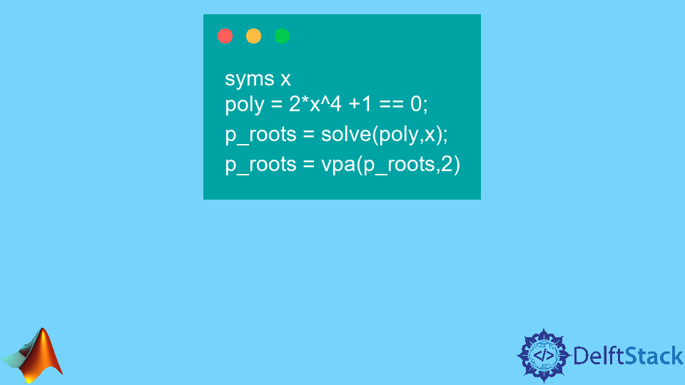
If you want to find the roots of a polynomial, you can use the solve() function in MATLAB. This input of this function is a polynomial. The output of this function is a column vector that contains the real and imaginary roots of the given polynomial. For example, let’s find the roots of a quadratic polynomial: 2x^2 — 3x + 6 = 0. We have to define the polynomial. See the code below.
poly = x^ x ;p_roots = solve(poly,x)p_roots = vpa(p_roots,) In the above code, we defined the whole polynomial, and we used the vpa() function to change the precision of the result. You can change the polynomial according to the given polynomial and the precision according to your requirements. Know, let’s find the roots of a quartic polynomial: 2x^4 + 1 = 0. See the code below.
poly = x^ ;p_roots = solve(poly,x);p_roots = vpa(p_roots,) - 0.59 - 0.59i - 0.59 + 0.59i 0.59 - 0.59i 0.59 + 0.59iIn the above code, we defined the whole polynomial and used the vpa() function to change the result’s precision. You can change the polynomial according to the given polynomial and the precision according to your requirements.
Получите корни полинома с помощью функции solve() в MATLAB
Если вы хотите найти корни многочлена, вы можете использовать функцию resolve() в MATLAB. Этот вход этой функции является полиномом. Результатом этой функции является вектор-столбец, содержащий действительные и мнимые корни данного многочлена. Например, давайте найдем корни квадратного многочлена: 2x ^ 2 — 3x + 6 = 0. Нам нужно определить многочлен. См. Код ниже.
poly = x^ x ;p_roots = solve(poly,x)p_roots = vpa(p_roots,) В приведенном выше коде мы определили весь многочлен и использовали функцию vpa(), чтобы изменить точность результата. Вы можете изменить полином в соответствии с заданным полиномом и точностью в соответствии с вашими требованиями. Знаем, давайте найдем корни многочлена четвертой степени: 2x ^ 4 + 1 = 0. См. Код ниже.
poly = x^ ;p_roots = solve(poly,x);p_roots = vpa(p_roots,) - 0.59 - 0.59i - 0.59 + 0.59i 0.59 - 0.59i 0.59 + 0.59iВ приведенном выше коде мы определили весь многочлен и использовали функцию vpa() для изменения точности результата. Вы можете изменить полином в соответствии с заданным полиномом и точностью в соответствии с вашими требованиями.
Solving System of Equations in Octave
We have a little different approach to solve a system of ‘n’ linear equations in ‘n’ unknowns. Let us take up a simple example to demonstrate this use.
Let us solve the equations −
5x + 9y = 5
3x – 6y = 4
Such a system of linear equations can be written as the single matrix equation Ax = b, where A is the coefficient matrix, b is the column vector containing the right-hand side of the linear equations and x is the column vector representing the solution as shown in the below program −
A = [5, 9; 3, -6];
b = [5;4];
A \ b
ans = 1.157895 -0.087719
In same way, you can solve larger linear systems as given below −
x + 3y -2z = 5
3x + 5y + 6z = 7
2x + 4y + 3z = 8
Solving Higher Order Equations in MATLAB
The solve function can also solve higher order equations. For example, let us solve a cubic equation as (x-3)2(x-7) = 0
solve('(x-3)^2*(x-7)=0')ans = 3 3 7
eq = 'x^4 - 7*x^3 + 3*x^2 - 5*x + 9 = 0';
s = solve(eq);
disp('The first root is: '), disp(s(1));
disp('The second root is: '), disp(s(2));
disp('The third root is: '), disp(s(3));
disp('The fourth root is: '), disp(s(4));
% converting the roots to double type
disp('Numeric value of first root'), disp(double(s(1)));
disp('Numeric value of second root'), disp(double(s(2)));
disp('Numeric value of third root'), disp(double(s(3)));
disp('Numeric value of fourth root'), disp(double(s(4)));
The first root is: 6.630396332390718431485053218985 The second root is: 1.0597804633025896291682772499885 The third root is: - 0.34508839784665403032666523448675 - 1.0778362954630176596831109269793*i The fourth root is: - 0.34508839784665403032666523448675 + 1.0778362954630176596831109269793*i Numeric value of first root 6.6304 Numeric value of second root 1.0598 Numeric value of third root -0.3451 - 1.0778i Numeric value of fourth root -0.3451 + 1.0778i
Please note that the last two roots are complex numbers.
Solving Quadratic Equations in MATLAB
The solve function can also solve higher order equations. It is often used to solve quadratic equations. The function returns the roots of the equation in an array.
eq = 'x^2 -7*x + 12 = 0';
s = solve(eq);
disp('The first root is: '), disp(s(1));
disp('The second root is: '), disp(s(2));
The first root is: 3 The second root is: 4
Expanding and Collecting Equations in Octave
When you work with many symbolic functions, you should declare that your variables are symbolic but Octave has different approach to define symbolic variables. Notice the use of Sin and Cos, which are also defined in symbolic package.
% first of all load the package, make sure its installed.
pkg load symbolic
% make symbols module available
symbols
% define symbolic variables
x = sym ('x');
y = sym ('y');
z = sym ('z');
% expanding equations
expand((x-5)*(x+9))
expand((x+2)*(x-3)*(x-5)*(x+7))
expand(Sin(2*x))
expand(Cos(x+y))
% collecting equations
collect(x^3 *(x-7), z)
collect(x^4*(x-3)*(x-5), z)
ans = -45.0+x^2+(4.0)*x ans = 210.0+x^4-(43.0)*x^2+x^3+(23.0)*x ans = sin((2.0)*x) ans = cos(y+x) ans = x^(3.0)*(-7.0+x) ans = (-3.0+x)*x^(4.0)*(-5.0+x)
Factorization and Simplification of Algebraic Expressions
Example
syms x
syms y
factor(x^3 - y^3)
factor([x^2-y^2,x^3+y^3])
simplify((x^4-16)/(x^2-4))
ans = (x - y)*(x^2 + x*y + y^2)
ans = [ (x - y)*(x + y), (x + y)*(x^2 - x*y + y^2)]
ans = x^2 + 4
Solving Basic Algebraic Equations in MATLAB
The solve function is used for solving algebraic equations. In its simplest form, the solve function takes the equation enclosed in quotes as an argument.
For example, let us solve for x in the equation x-5 = 0
solve('x-5=0')ans = 5
You can also call the solve function as −
y = solve('x-5 = 0')y = 5
You may even not include the right hand side of the equation −
solve('x-5')ans = 5
If the equation involves multiple symbols, then MATLAB by default assumes that you are solving for x, however, the solve function has another form −
solve(equation, variable)
where, you can also mention the variable.
For example, let us solve the equation v – u – 3t2 = 0, for v. In this case, we should write −
solve('v-u-3*t^2=0', 'v')ans = 3*t^2 + u
Solving System of Equations in MATLAB
The solve function can also be used to generate solutions of systems of equations involving more than one variables. Let us take up a simple example to demonstrate this use.
Let us solve the equations −
5x + 9y = 5
3x – 6y = 4
s = solve('5*x + 9*y = 5','3*x - 6*y = 4');
s.x
s.y
ans = 22/19 ans = -5/57
x + 3y -2z = 5
3x + 5y + 6z = 7
2x + 4y + 3z = 8
Получите корни многочлена с помощью функции roots() в MATLAB
Если вы хотите найти корни многочлена, вы можете использовать функцию roots() в MATLAB. Этот вход этой функции — вектор, который содержит коэффициенты полинома. Если в полиноме нет степени, то в качестве его коэффициента будет использоваться 0. Результатом этой функции является вектор-столбец, содержащий действительные и мнимые корни данного многочлена. Например, давайте найдем корни квадратного полинома: 2x ^ 2 — 3x + 6 = 0. Мы должны определить коэффициенты полинома, начиная с наивысшей степени, и если степень отсутствует, мы будем использовать 0 в качестве ее коэффициента. . См. Код ниже.
p_roots = roots(poly) 0.7500 + 1.5612i 0.7500 - 1.5612iВ приведенном выше коде мы использовали только коэффициенты полинома, начиная с наибольшей степени. Вы можете изменить коэффициенты многочлена в соответствии с данным многочленом. Знаем, давайте найдем корни многочлена четвертой степени: 2x ^ 4 + 1 = 0. См. Код ниже.
p_roots = roots(poly) -0.5946 + 0.5946i -0.5946 - 0.5946i 0.5946 + 0.5946i 0.5946 - 0.5946iМы использовали три 0 между двумя полиномами в приведенном выше коде, потому что три степени отсутствуют. Проверьте эту ссылку для получения дополнительной информации о функции root().
Get the Roots of the Polynomial Using the roots() Function in MATLAB
If you want to find the roots of a polynomial, you can use the roots() function in MATLAB. This input of this function is a vector that contains the coefficients of the polynomial. If a power is not present in the polynomial, then 0 will be used as its coefficient. The output of this function is a column vector that contains the real and imaginary roots of the given polynomial. For example, let’s find the roots of a quadratic polynomial: 2x^2 — 3x + 6 = 0. We have to define the polynomial coefficients starting from the highest power, and if a power is not present, we will use 0 as its coefficient. See the code below.
p_roots = roots(poly) 0.7500 + 1.5612i 0.7500 - 1.5612iIn the above code, we only used the coefficients of the polynomial starting from the highest power. You can change the coefficients of the polynomial according to the given polynomial. Know, let’s find the roots of a quartic polynomial: 2x^4 + 1 = 0. See the code below.
p_roots = roots(poly) -0.5946 + 0.5946i -0.5946 - 0.5946i 0.5946 + 0.5946i 0.5946 - 0.5946iSolving Quadratic Equations in Octave
s = roots([1, -7, 12]);
disp('The first root is: '), disp(s(1));
disp('The second root is: '), disp(s(2));
The first root is: 4 The second root is: 3
Expanding and Collecting Equations in MATLAB
When you work with many symbolic functions, you should declare that your variables are symbolic.
syms x %symbolic variable x
syms y %symbolic variable x
% expanding equations
expand((x-5)*(x+9))
expand((x+2)*(x-3)*(x-5)*(x+7))
expand(sin(2*x))
expand(cos(x+y))
% collecting equations
collect(x^3 *(x-7))
collect(x^4*(x-3)*(x-5))
ans = x^2 + 4*x - 45
ans = x^4 + x^3 - 43*x^2 + 23*x + 210
ans = 2*cos(x)*sin(x)
ans = cos(x)*cos(y) - sin(x)*sin(y)
ans = x^4 - 7*x^3
ans = x^6 - 8*x^5 + 15*x^4
Solving Higher Order Equations in Octave
v = [1, -7, 3, -5, 9];
s = roots(v);
% converting the roots to double type
disp('Numeric value of first root'), disp(double(s(1)));
disp('Numeric value of second root'), disp(double(s(2)));
disp('Numeric value of third root'), disp(double(s(3)));
disp('Numeric value of fourth root'), disp(double(s(4)));
Numeric value of first root 6.6304 Numeric value of second root -0.34509 + 1.07784i Numeric value of third root -0.34509 - 1.07784i Numeric value of fourth root 1.0598
Solving Basic Algebraic Equations in Octave
For example, let us solve for x in the equation x-5 = 0
roots([1, -5])
ans = 5
You can also call the solve function as −
y = roots([1, -5])
y = 5
How To Use ‘roots()’ Command In Matlab®?
>> a = [5 6 8 4 3];
roots(a)
ans = -0.5866 + 0.7505i -0.5866 - 0.7505i -0.0134 + 0.8130i -0.0134 - 0.8130i
>>
First of all, you need to know how to define polynomials in Matlab®. To define a polynomial, you need to create a vector that represents this polynomial in Matlab®. For example, we created a vector called ‘a’ as shown above, that represents the polynomial of 5x^4+6x^3+8x^2+4x+3. As you understand that each of the coefficients is represented by an element in’ vector, from right to left. So, the logic behind the definition of polynomials in Matlab is this.
YOU CAN LEARN MatLab® IN MECHANICAL BASE; Click And Start To Learn MatLab®!
Calculation of roots of a polynomial in Matlab® is very easy actually. To calculate the roots of polynomials in Matlab®, you need to use theroots()’ command. As you see above example, we calculated the roots of polynomial ‘a’. What we did is just typing the ‘a’ inside the parenthesis of the ‘roots()’ command as shown above. As you see that the result has four roots. All the roots of this polynomial are complex numbers.
Finding or calculating roots of a polynomial with the ‘roots()’ command in Matlab® is very easy like above.
Conclusion
Do not forget to leave your comments and questions about the ‘roots()’ command in Matlab® below. Your feedback is very important for us.
This article is prepared for completely educative and informative purposes. Images used courtesy of Matlab®
Your precious feedbacks are very important to us.
")


")